Pivot tables are perhaps one of the most important data presentation tools that a spreadsheet application can have. The focus word here is presentation.
A default pivot table can have bland features that do not convey the data clearly most of the time.
That’s where formatting becomes crucial. And in this article, we will look at a few ways we can perform pivot table formatting in Google Sheets.
Let’s get started.
Formatting a Pivot Table in Google Sheets
First things first, let’s create a pivot table in Google Sheets. Here we have a sample dataset of sales data according to month and region:
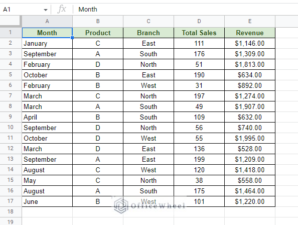
We will create a pivot table that focuses on presenting the number of sales in each month by product.
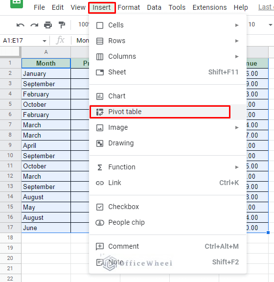
Step 1: Select the whole dataset and navigate to the Insert tab to find the Pivot table option.
Insert > Pivot Table
Step 2: Set the following conditions in the Pivot Table Editor as seen in the image below:
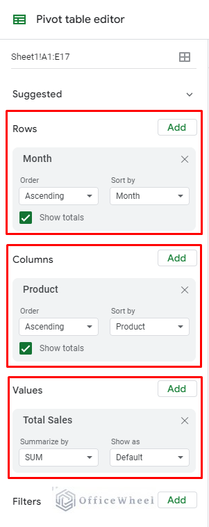
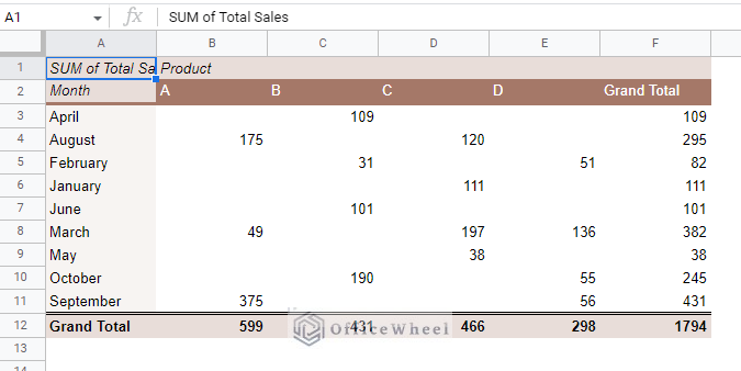
And we are done!

This is the default look of any pivot table in Google Sheets. While it conveys the message just fine, it is not quite presentable.
To make it so, we will use some formatting techniques that are already available in the application and are quite easy to use.
1. Using Predefined Themes to Format a Pivot Table in Google Sheets
The easiest way to bring life to your pivot table is to use themes. Thankfully, Google Sheets already provides us with a set of predefined themes right in the application.
We can easily find the option in the Format tab.
Format > Theme
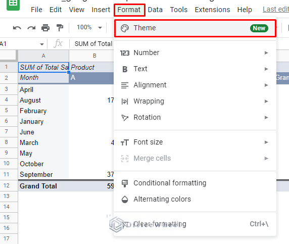
This will open the Themes pane on the right-hand side of the window.
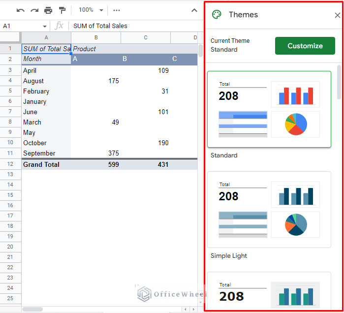
As you can see, there are a plethora of options to choose from. Select the one that closely matches the data or your presentation.
Customize Themes
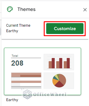
While the number and variety of the themes available are respectable, Google Sheets further allows us to customize them to format the pivot table in any way we want.
You will find the Customize button on the Themes pane. After settling on a general theme, click on the button to get started.
Clicking on the button will open a general customization panel. Here you can set your pivot table to have any fonts or any color that you desire for the different aspects of a dataset presented here.
Click Done to finish up.
2. Format a Pivot Table Manually
Fundamentally, a pivot table is simply a generated table from a source dataset in Google Sheets. This means that any customizations you can do in a regular worksheet can also be performed on a pivot table.
For example, let’s say we want to…
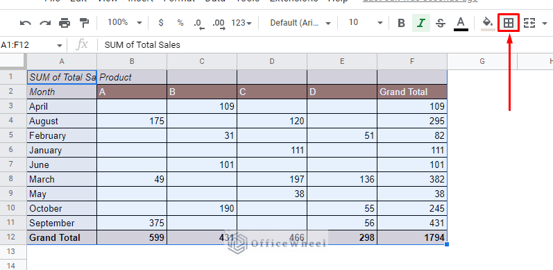
- Apply a border to the table
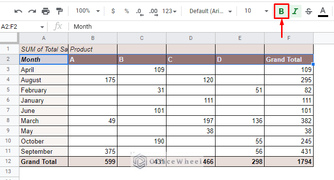
- Bold the column headers
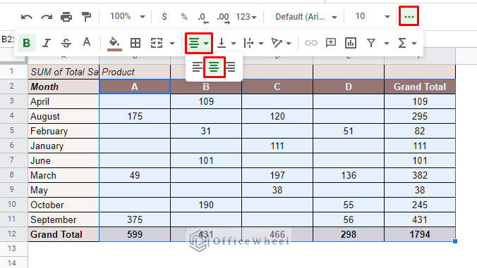
- Center-align the column headers and data
Of the following pivot table in Google Sheets:
We will take the same steps for this formatting as we would for a regular worksheet.
- Applying a border: Select the table and click on the Border icon on the ribbon.
- Bold text: Select the text, in this case, the column headers, and click on the Bold icon on the Ribbon. You can also use the keyboard shortcut CTRL+B.
- Center-align the data and headers: Select the data and header cells and click on the Alignment button to open the tray and select Center.
These are just a few examples of manual formatting. There’s so much more available in Google Sheets.
3. Conditional Formatting a Pivot Table in Google Sheets
Same as manual formatting, we can also apply conditional formatting to a pivot table in Google Sheets.
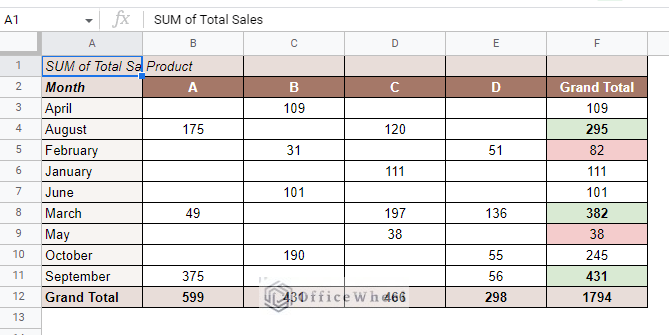
For this example, let’s highlight the Grand Total of Sales for each month. Sales above 250 units get one highlight and sales under 100 units another highlight.
Step 1: Select the cell to highlight.
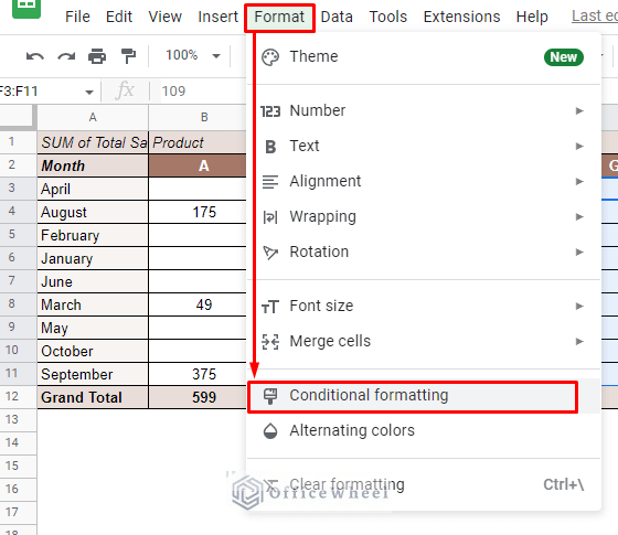
Step 2: Navigate to Conditional formatting from the Format tab.
Format > Conditional formatting
Step 3: Apply the first conditional formatting to values above 250.
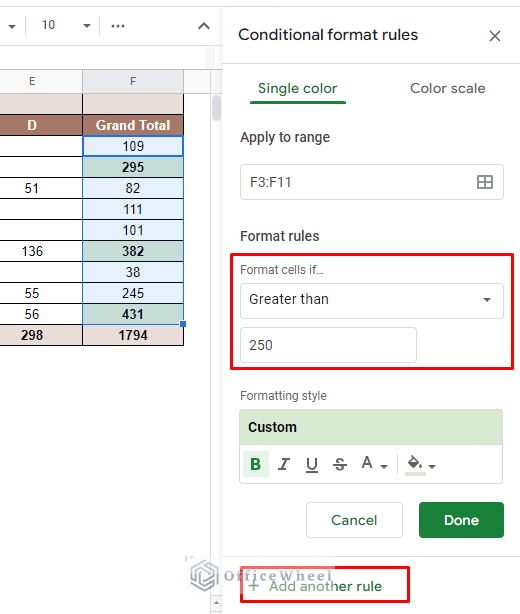
Click Add another rule for the second conditional format.
Step 4: Apply the second conditional formatting to values under 100.
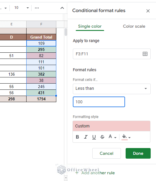
Step 5: Click Done to apply.
Learn More: How to Use Conditional Formatting in Google Sheets
Final Words
That concludes all the ways you can format a pivot table in Google Sheets. Themes are specially made to be applied to these tables in the application, they can also be customized according to the users’ requirements.
Other than themes, a user can apply any type of formatting that is already available in Google Sheets on a pivot table. That includes conditional formatting.
Feel free to leave any queries or advice you might have for us in the comments section below.