When we think about multiple conditions, the first thing that comes to mind is its logical formatting. So it comes to no surprise that when creating custom formulas for conditional formatting with multiple conditions in Google Sheets, we primarily use the OR and AND logical operations.
3 Ways to Use Conditional Formatting with Multiple Conditions in Google Sheets
1. Using OR Logic
We start with the OR logical condition. The logic states that, even if one condition is TRUE, the whole formula will be considered as a TRUE statement.
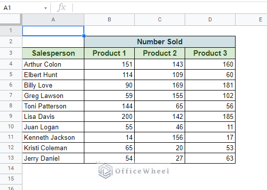
For our example, we will highlight the Names of the employees that have a Sales Number under 50 in at least one Product from the following dataset.
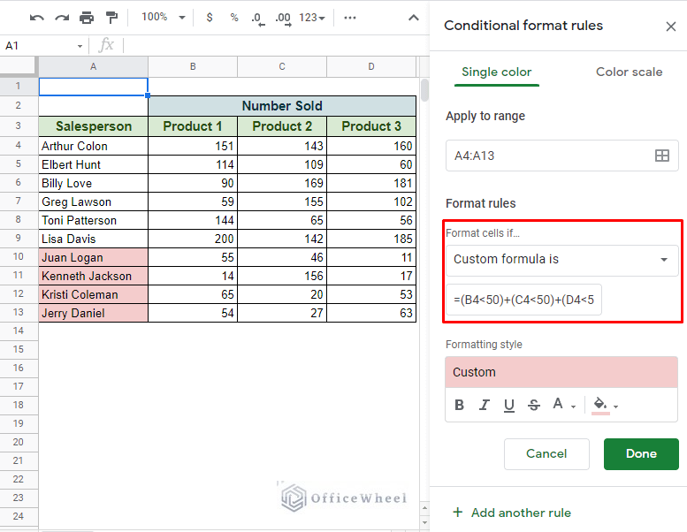
The simplest way to use the OR logic is by using the addition operator (+) in between the conditions. So, in the custom formula field, we enter the formula:
=(B4<50)+(C4<50)+(D4<50)If you want to know how to apply custom formulas in conditional formatting, please visit our Using Conditional Formatting With Custom Formula in Google Sheets article.
Condition Breakdown:
- Our data range that was chosen is only the Salesperson column (A4:A13) to highlight only names. See Apply to range section in the image.
- Each condition corresponds to a Product column, so we have three conditions for three columns.
Alternatively, we can also use the OR function to get the same result:
=OR(B4<50,C4<50,D4<50)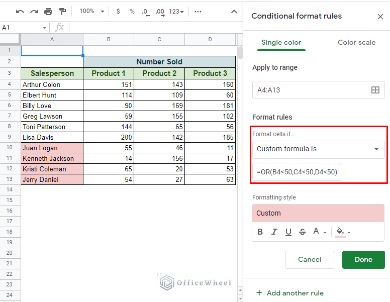
On top of being concise, the OR function allows users to use it in various formulas which we will see later in this article.
That concludes the fundamental way to use the OR logic to use conditional formatting with multiple conditions in Google Sheets
OR Alternative: Add Another Rule Option
The conditional formatting window of Google Sheets allows us to add more conditions to our selected data range. While the uses may be limited, it still mimics much of the OR logic that we have just discussed.
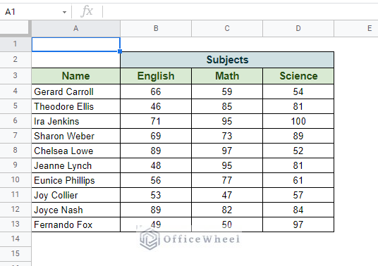
Let’s say we want to highlight all the marks under 60 with one color and all the marks above 90 with another from the following table.
These are essentially two separate conditions that can be applied directly from the Conditional format rules window.
First of all, let’s select the range of formatting. Since we only want to highlight the marks our data range will be B4:D13.
Then we add our first condition as a custom formula to highlight all the marks under 60.
=B4<60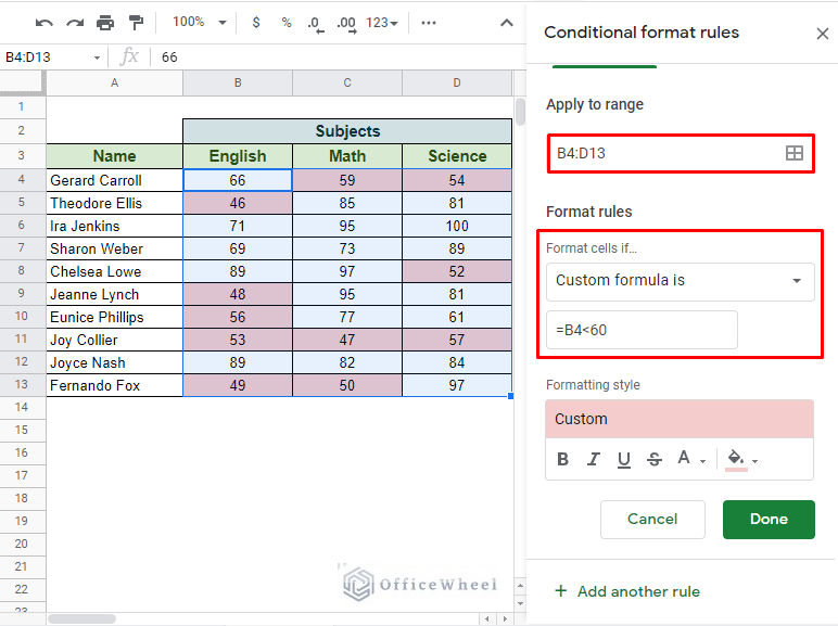
The Formatting style will be of your choice.
Now, notice the Add another rule option at the bottom of the window.
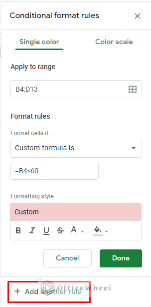
Clicking on it will take us to a fresh window with most of the conditions the same as before. Add the second condition for our task, that is, highlighting all the marks greater than 90 but with a different color.
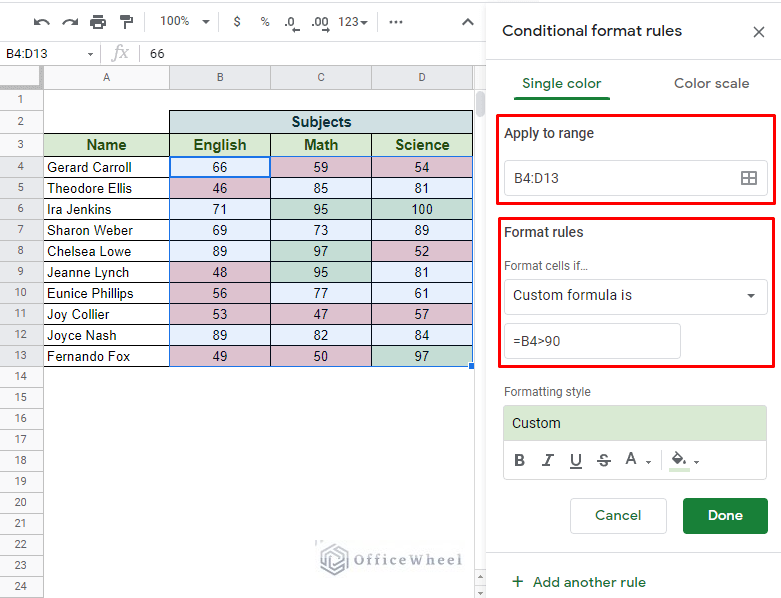
This process is essentially applying two different conditions on the same range in conditional formatting in Google Sheets. Just make sure that the condition range does not overlap.
Read More: Conditional Formatting with Multiple Conditions Using Custom Formulas in Google Sheets
2. Using AND Logic
The AND logic follows similar syntaxes as the OR function, only this time, instead of the plus operator (+) we will use the multiplication operator or asterisk (*).
For a refresher: The AND logic will return TRUE only if all the conditions are TRUE.
So, coming back to our initial dataset, we will apply the conditional formatting condition to highlight the names that have achieved more than 100 sales in all three products.
Our first AND logic formula:
=(B4>100)*(C4>100)*(D4>100)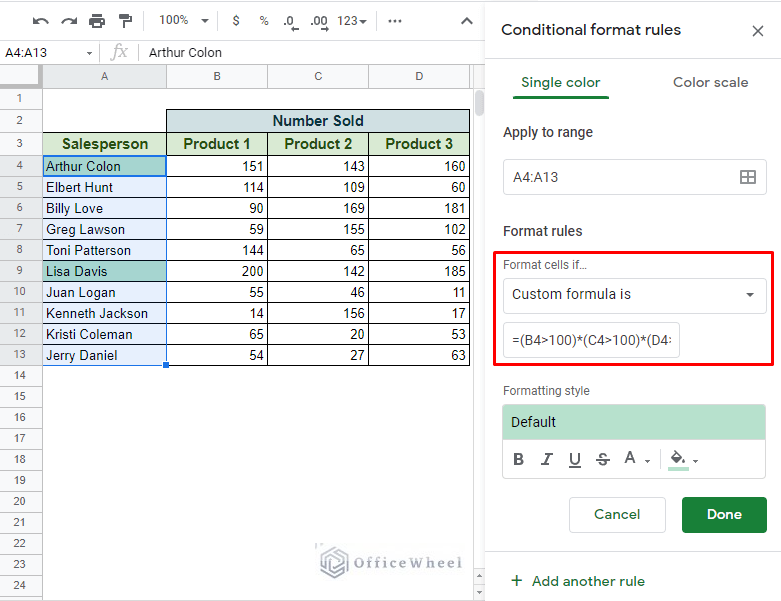
And of course, there is an AND function alternative:
=AND(B4>100,C4>100,D4>100)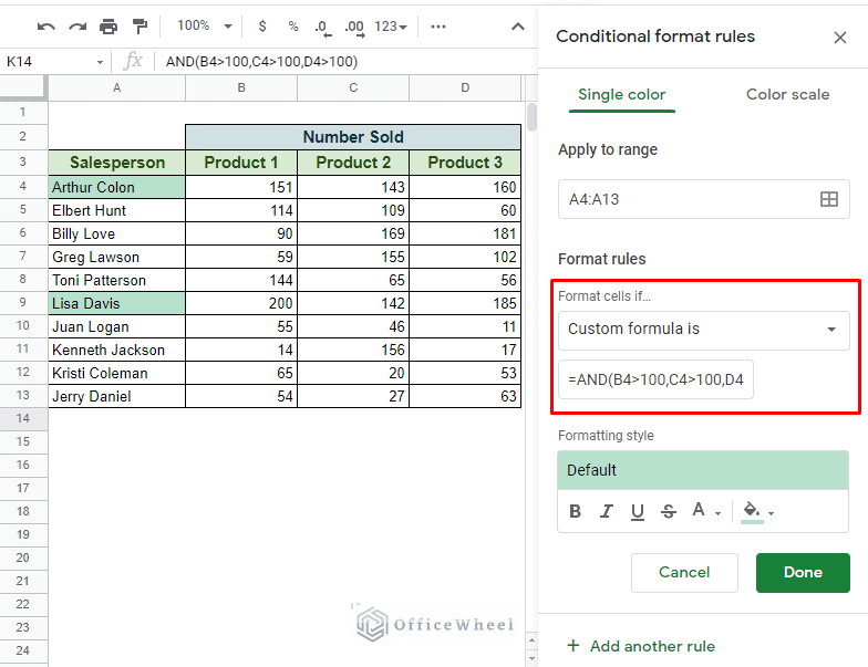
AND-OR Combination
The main advantage of using functions is the ability to combine them to extract more complex results. That is what we are going to do with the AND and OR functions.
For this example, we will use conditional formatting to highlight the rows that have an Amount Sold value of over 300 units and are in the Location of New York or Philadelphia from the following dataset.
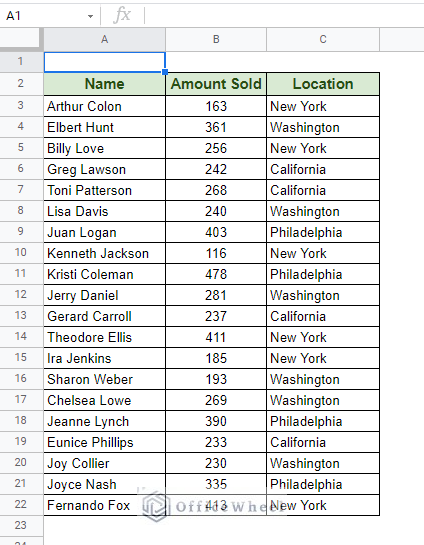
Our custom combined formula for conditional formatting is:
=AND($B3>300,OR($C3="New York",$C3="Philadelphia"))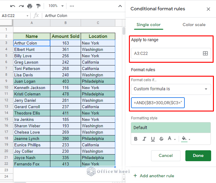
Notice that we have used all the value cells from our table for our formatting range, A3:C22.
Read More: Highlight Row If Cell Contains Text with Conditional Formatting in Google Sheets
Similar Readings
- Conditional Formatting with Checkbox in Google Sheets
- Match Multiple Values in Google Sheets (An Easy Guide)
- How to Use Nested IF Function in Google Sheets (4 Helpful Ways)
- Change Row Color Based on Cell Value in Google Sheets (4 Ways)
- Copy Formatting From One Sheet To Another In Google Sheets (2 Ways)
3. Using the COUNTIFS Function (Situational)
The situation is highlighting duplicates in Google Sheets, but this time with multiple conditions.
Generally, we use the COUNTIF function to highlight duplicates in a single column, however, for multiple conditions or columns, we have to utilize the COUNTIFS function.
Let’s keep things simple. From the following dataset, we will highlight all the rows where both columns have duplicate entries.
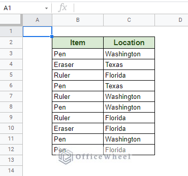
Our formula:
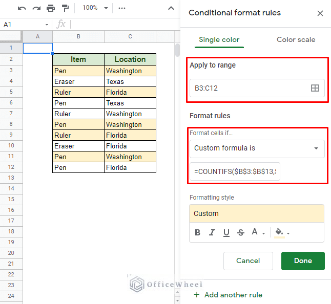
Read More: How to Highlight Duplicates for Multiple Columns in Google Sheets
Final Words
That concludes all the ways we can use conditional formatting with multiple conditions in Google Sheets. We hope that the methods we have discussed come in handy for your spreadsheet tasks.
Feel free to leave any queries or advice you might have for us in the comments section below.
Related Articles
- Conditional Formatting Based on Another Cell in Google Sheets
- Pivot Table Formatting in Google Sheets (3 Easy Ways)
- How to Copy Conditional Formatting in Google Sheets
- Use REGEXMATCH Function for Multiple Criteria in Google Sheets
- How to Use IF and OR Formula in Google Sheets (2 Examples)
- How to Search in All Sheets in Google Sheets (An Easy Guide)
- Google Sheets: Highlight Row If Cell Is Empty