Highlight Row If Cell Contains Text with Conditional Formatting in Google Sheets

While working with data in Google Sheets you may sometimes need to highlight the entire row containing data in a particular cell. Doing this manually without any formula may be tiring and time-consuming if you have a large amount of data. In this article, we will try to show you how you can use conditional formatting to highlight row if cell contains text in Google Sheets easily.

Table of Contents

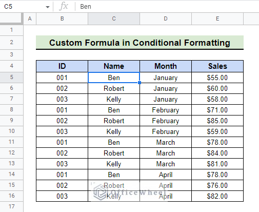
A Sample of Practice Spreadsheet

Highlight Row If Cell Contains Text

2 Ways to Use Conditional Formatting to Highlight Row If Cell Contains Text in Google Sheets

1. Using Custom Formula in Conditional Formatting

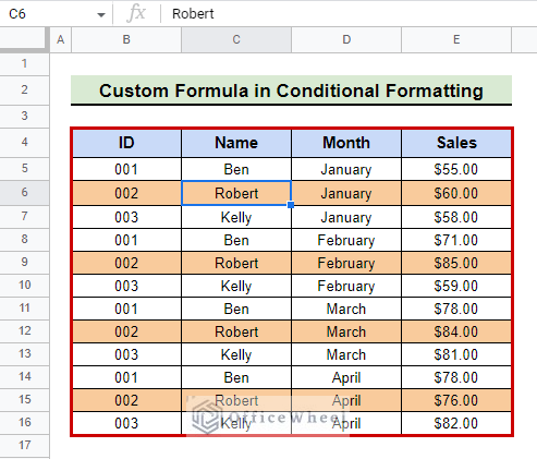
We’ll begin with a simple example that highlights the row if the cell contains text. In our example, we use a data table with employee ID, Names, Months, and monthly Sales amount.

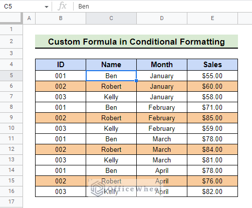
We will highlight the row containing the name Robert in the table using Conditional formatting. For this to work, we need to introduce a formula that we discussed later.

Conditional formatting will highlight the entire row if it can find the name Robert in any of the cells.

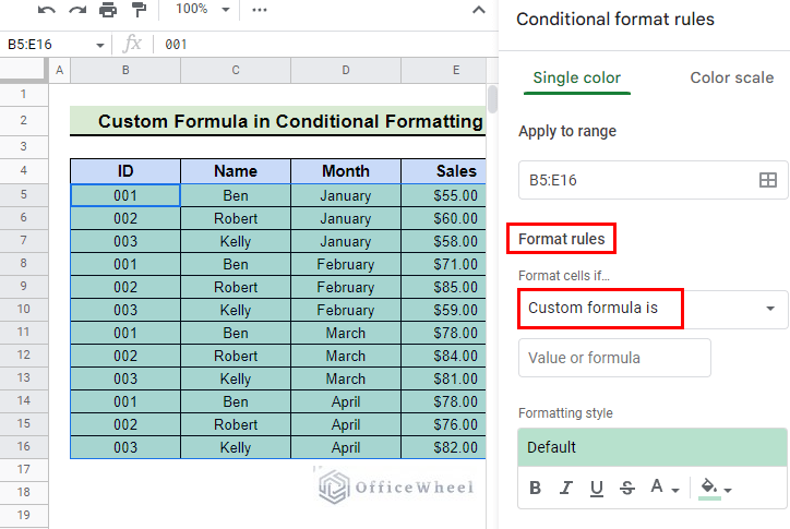
The steps you need to follow:

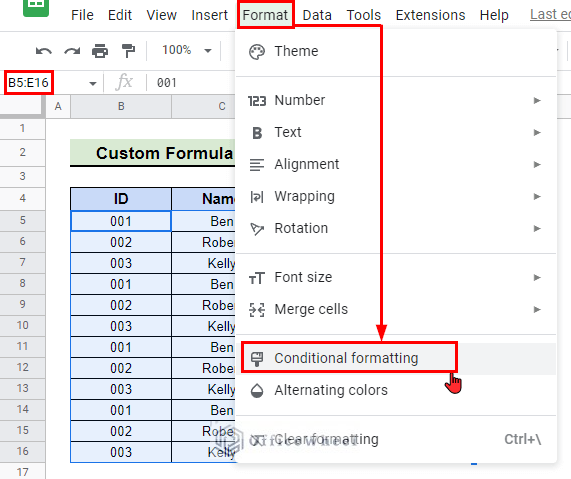
First, open the spreadsheet and select the range of tables where you want the highlight to take place. We select the range B5:E16.
Then, go to Menu bar > Format > Conditional formatting.

You will see a Conditional formatting sidebar appear from the right side. The sidebar specifies where it is applying the Conditional formatting in the Apply to range In our example, it says B5:E16.

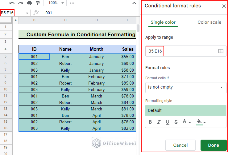
Next, from the Format rules tab from Format cells if box select Custom Formula is option because by default the Conditional formatting is applied to all the cells having any text or values and we do not want that.

Then, in the Value or formula box type in the following formula:

=$C5="Robert"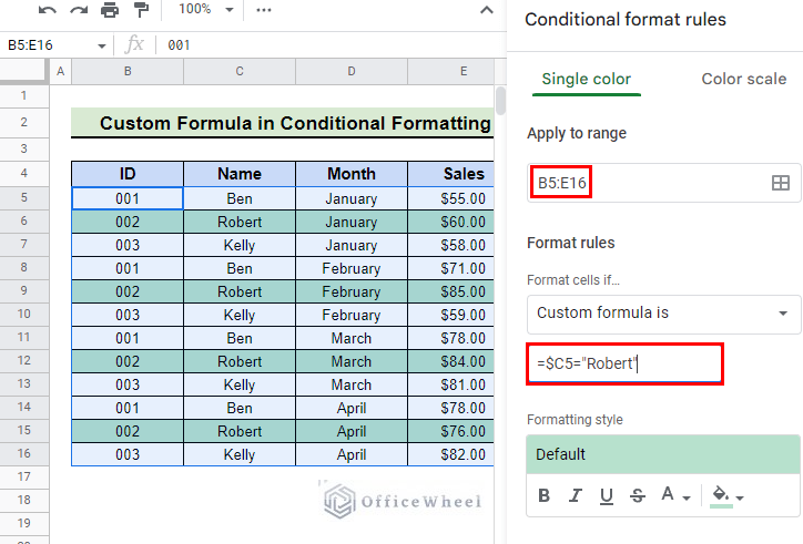

Formula Explanation:

The first part of the formula $C5 determines where the name Robert is in the table and tells Sheets to start matching from that cell. Notice how C is locked with a dollar($) sign and 5 is not. This is because we do not want the column value to change but to keep the row value flexible when conditional formatting looks across the entire table.
The second part of the formula “Robert” is the condition the Conditional formatting has to meet to highlight. If it is an exact match then the entire row will be highlighted, otherwise it will remain as is.

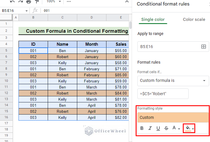
You can format the highlighted table further in the Formatting style You can select a custom font size and even select a preferred color. We select light orange 2 for our example.

Finally, press Done and you can see the rows highlighted.

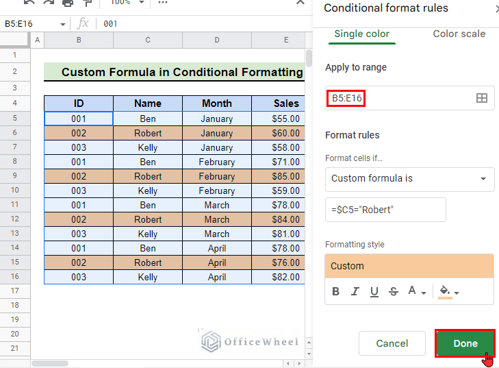
This is how the final dataset looks:

2. Applying REGEXMATCH Function for Partial Text Match

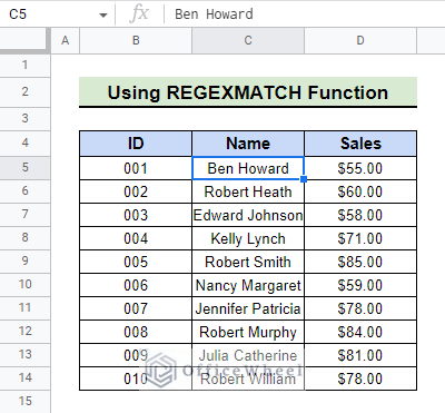
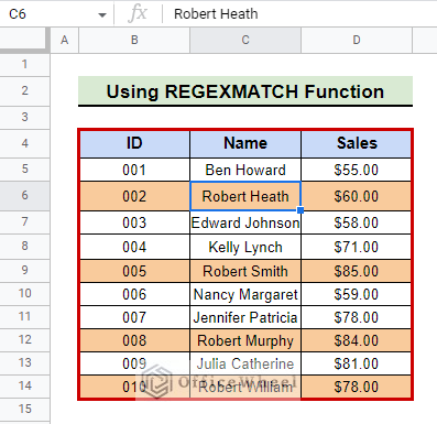
REGEXMATCH can be used with Conditional formatting to highlight row if the cell contains text without much hassle. For this, we use a data table with employee ID, Names, and monthly Sales amount. We will apply the REGEXMATCH function to highlight the row for all the first names containing Robert.

Follow these steps:

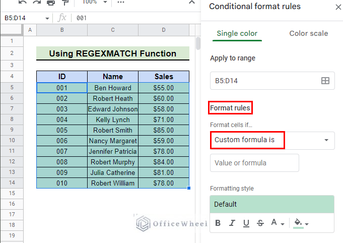
First, open the spreadsheet and select the range of tables where you want the highlight to take place. We select the range B5:D14.
Then, go to Menu bar > Format > Conditional formatting.

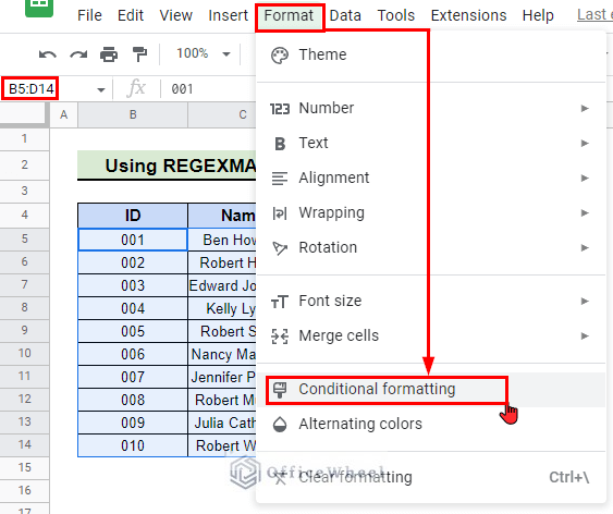
You will see a Conditional formatting sidebar appear from the right side.
The sidebar specifies where it is applying the Conditional formatting in the Apply to range In our example, it says B5:D14.

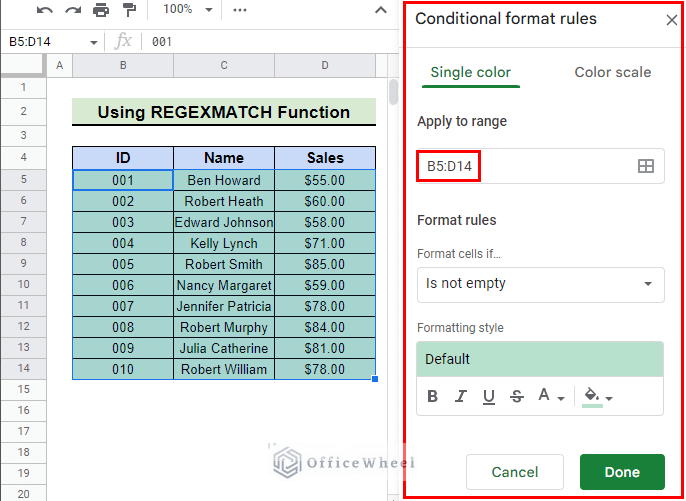
Next, from the Format rules tab from Format cells if box, select Custom Formula is option because by default the Conditional formatting is applied to all the cells having any text or values and we do not want that.

Then, in the Value or formula box type in the following formula:

=REGEXMATCH($C5, "\ARobert\s")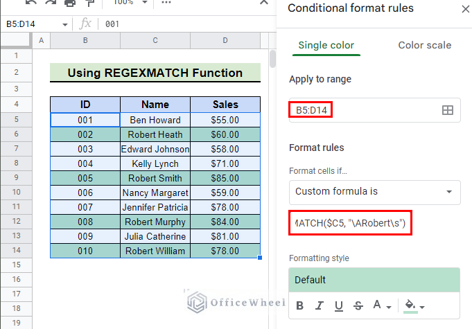

Formula Explanation:

The first part of the formula $C5 determines where the name Robert is in the table and tells Sheets to start matching from that cell. You can notice that C is locked with a dollar($) sign and 5 is not. This is because we do not want the column value to change but to keep the row value flexible when conditional formatting looks across the entire table.
The second part of the formula “\ARobert\s” is the condition the Conditional formatting has to meet to highlight. \A matches any letters from A-Z. If it matches the words Robert, then the entire row will be highlighted, otherwise, it will remain as is.
Notice how Conditional formatting does not look for the full name, but rather the first name Robert. REGEXMATCH made this possible
\s matches a whitespace character. In our case, the space between the first and last name.

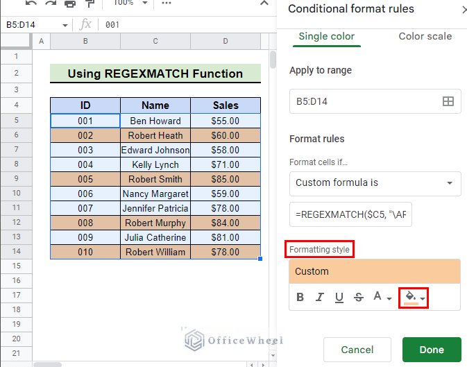
You can format the highlighted table further in the Formatting style You can select custom font size and even select a preferred color. We select light orange 2 for our example.

Finally, press Done and you should see the rows highlighted.

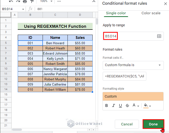
This is how the final dataset looks:

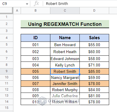
You can use the REGEXMATCH function to highlight the row for all the last names containing Smith For this, just type in the following formula:

=REGEXMATCH($C5, "\sSmith")

Follow the same steps as you did for the first name, only this time the \s is before the potential last name, in our case which is Smith.

Potential Problems, Solutions, and Tips

While trying to highlight a row with particular text, if you are not careful then you may not get the desired outcome.

Carefully select cells and use cell references properly. Use absolute cell references ($) when possible.
Make sure there is no other Conditional formatting overlapping the existing one.
Remove any unwanted extra spaces between words. For this, you can use the TRIM function.

Conclusion

In this article, we showed you how to use Conditional formatting to highlight row if a cell contains text in Google Sheets. We hope this article was useful to you. Keep practicing the methods that we have shown here to get a good grip on the concept.

Also, check out other articles on OfficeWheel to keep on improving your Google Sheets work knowledge.