Today we will have a look at how to use conditional formatting in Google Sheets, which is potentially one of the most used built-in functions by any level of spreadsheet user for data presentation or reports.
The Basics of Conditional Formatting in Google Sheets
Navigating to the Conditional Formatting Option
We start off by seeing how to navigate to and open the Conditional formatting window.
- Click on the Format tab on the top of the Toolbar.
- Select the Conditional formatting option.
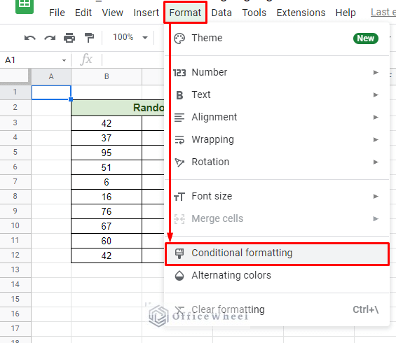
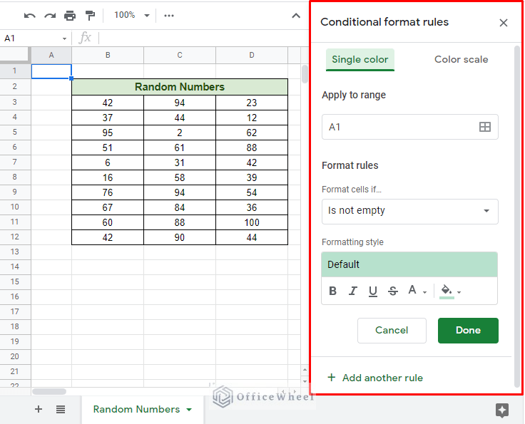
This should open the Conditional format rules window, from which you can apply conditional formatting to your Google Sheets worksheet.
The Two Modes
You may have noticed the two tabs at the top of the Conditional formatting rules window: Single color and Color scale.
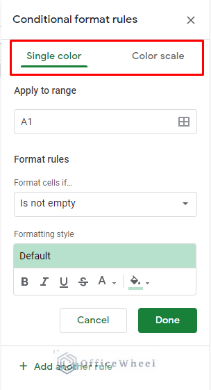
Single color mode
The Single color mode is the most commonly used. However, we should not overlook the ability or the many uses of the Color scale mode.
In this article, we will discuss these two modes in detail.
1. Conditional Formatting with Single Color in Google Sheets
The Three Sections
Let’s break down the Single color mode into three sections for better understanding:
- Apply to range
- Format rules
- Formatting Style
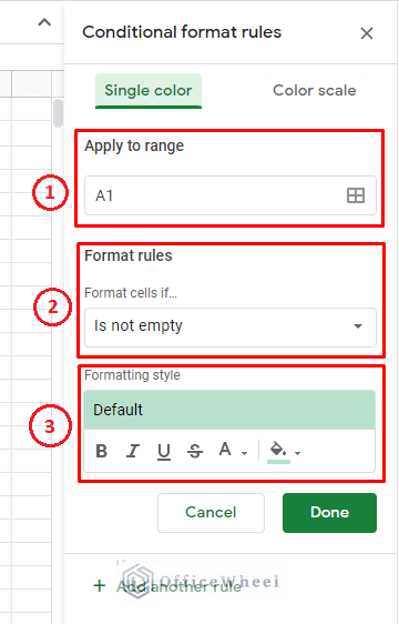
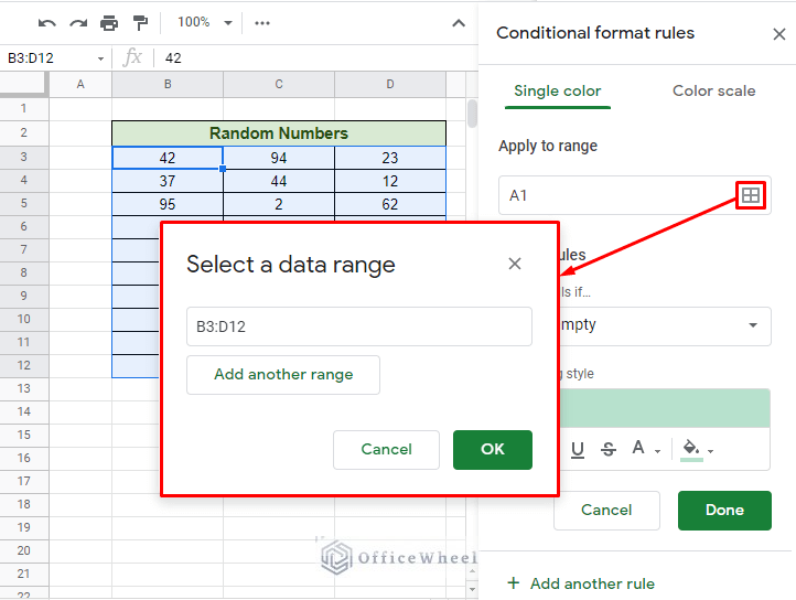
The Apply to range section determines the range of cells upon which the conditional formatting will be applied.
You can either select this range before opening the conditional formatting window, or you can input the range afterward by clicking on the ‘grid’ icon in this section.
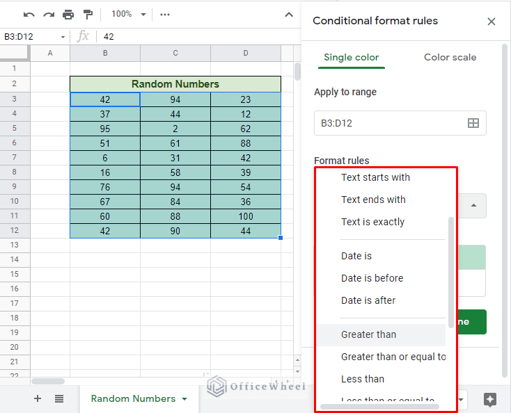
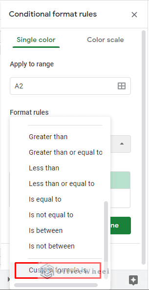
The Format rules section is where the bulk of our work happens. As you can see from the following image, we have a bunch of conditions (including custom formulas) that we can utilize to format our selected cells, which we will discuss more in detail in the Examples section.
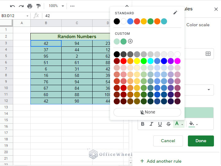
Finally, we have the Formatting style section. As you can see, here is where we customize how our cells and their data will transform according to the defined conditions.
How does Conditional Formatting work?
Conditional formatting works by evaluating whether the cells in the data range are TRUE or not according to the given condition (Format rules). If TRUE, the formatting style defined by the user will be applied. If not, nothing changes.
Examples With Different Format Rules
In this section, we will look at some examples of the many options available to us in the Format rules of conditional formatting. We have separated these rules into four different groups.
I. General and Text Conditions
Our first group for Format rules consists of general and text conditions.
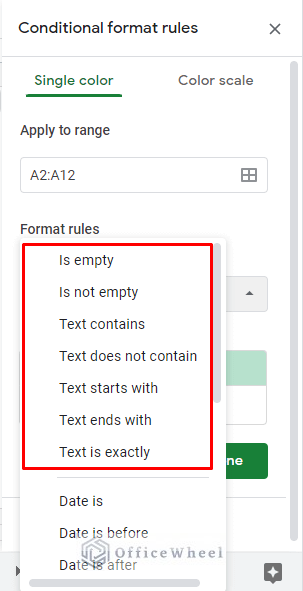
For example, if we choose the condition “is empty”, we get the following result, highlighting all the blank cells:

The opposite condition, “is not empty” can also be used to highlight all cells that contain values, either text or numbers.
On the other hand, the Text conditions act as you’d expect. You will have to input a text condition that will be utilized to match in the given range.
For example, we can apply the rule “Text starts with” and input the condition “T” to look for all the text instances that start with the letter T.
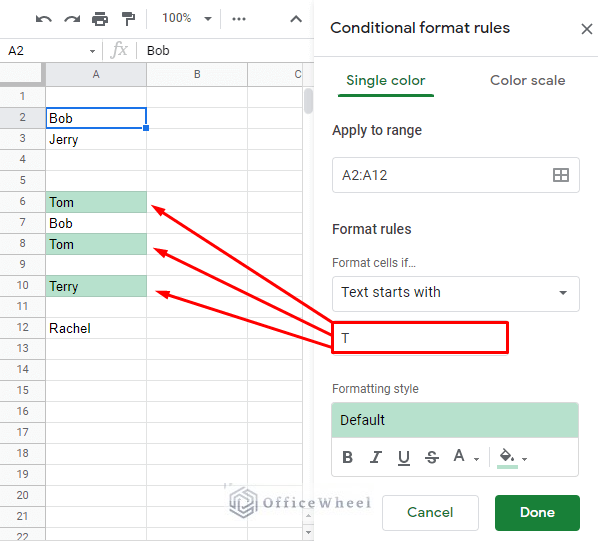
Note: The Text conditions are case insensitive. Case-sensitive conditions can be done with Custom Formulas.
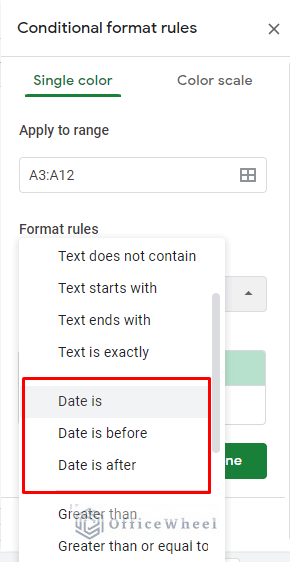
II. Date Conditions
Next, we have the Date Format rules.
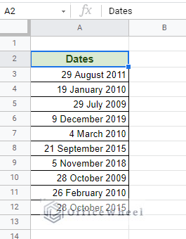
For example, let’s say we want to highlight all dates after 1 January 2011 from the following dataset:
Let’s go through the process step by step.
Step 1: Select the range of cells that you want to apply a conditional format to. For us, it is A3:A12.
Step 2: Select the “Date is after” format rule.
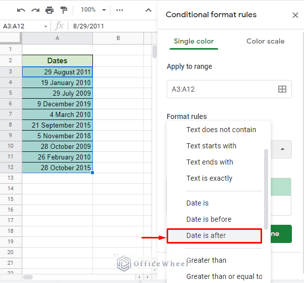
Here you will be presented with another set of rules. Select “exact date”.
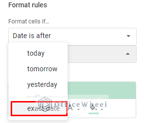
Enter the date 1 January 2011 and all the respective cells will be highlighted.
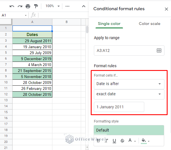
The other Date rules work in the same way.
III. Numerical Conditions
Numerical conditions are some of the most used rulesets in conditional formatting, and so too understandably.
Here we can see all the number rules available to us:
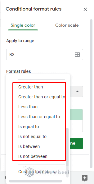
As you may have noticed, these are all logical conditions that can be used to highlight any numerical calculation.
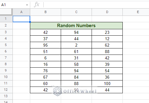
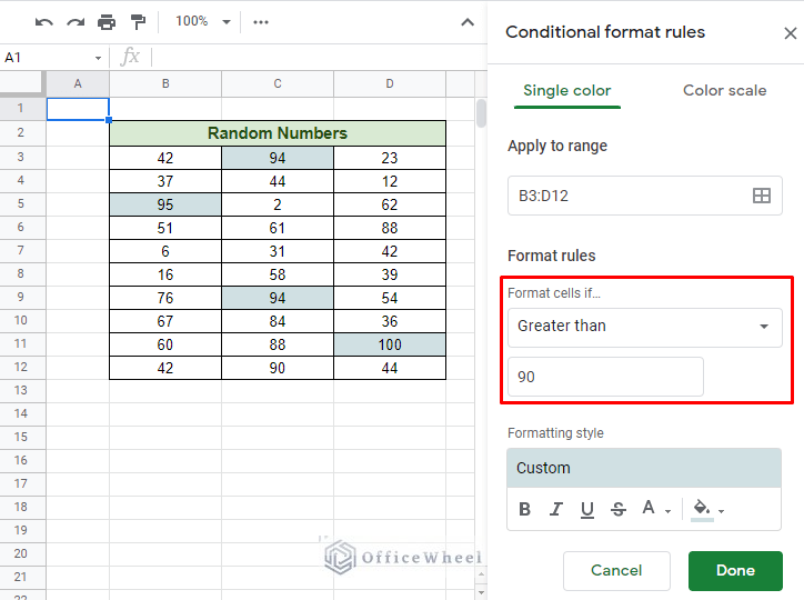
For example, let’s say we want to highlight all the numbers above 90 with one color and all the numbers under 20 with another from the following dataset.
Our first condition:
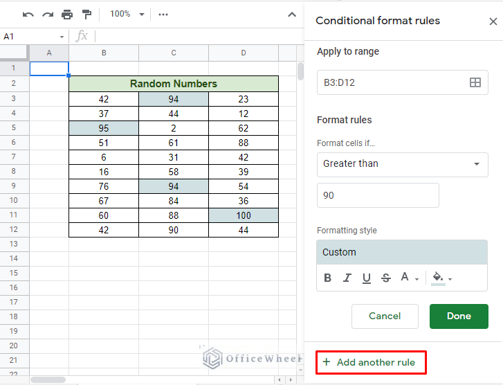
To add the second condition, scroll to the bottom of the Conditional format rules window and select Add another rule.
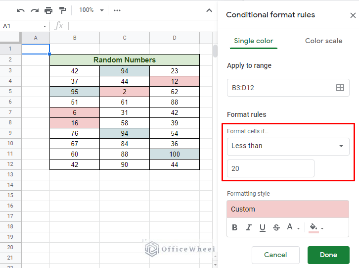
Our second condition:
IV. Custom Formulas
Till now, all the conditions that we have discussed are fairly basic, but conditional formatting wouldn’t be called such a powerful tool for these only.
The main selling point of conditional formatting comes from customization, and I am not talking about formatting.
The conditions for conditional formatting can be further enhanced by the use of custom formulas, which we can access from here (bottom of the drop-down menu):
One of the most common uses of custom formulas in conditional formatting is to highlight duplicates in a Google Sheets worksheet.
The formula is:
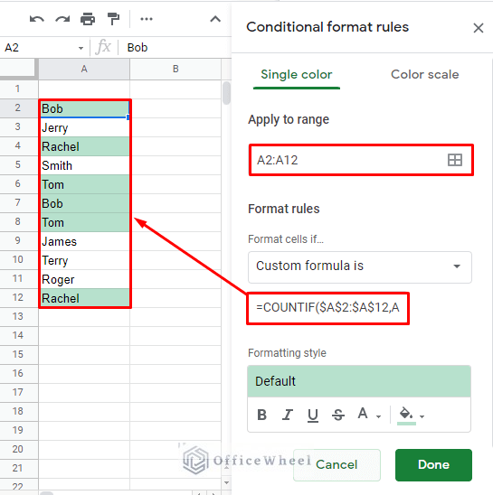
This is just one of the virtually endless examples of how to use custom formulas in conditional formatting in Google Sheets. The better you understand how functions work in Google Sheets, the better you can utilize the potential of custom formulas.
2. Conditional Formatting with Color Scale in Google Sheets
It’s time to have a look at the other conditional formatting mode, the Color Scale. With this, you can essentially heatmaps with scores and results in Google Sheets.
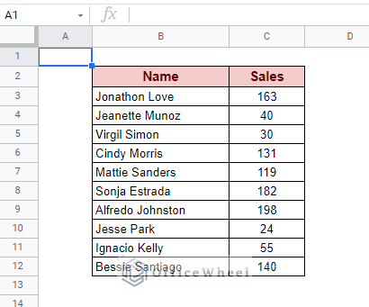
To show this process, we have created the following data set of the Name of salesmen and Sales of a shop. We will be highlighting the sales amount using the color scale of conditional formatting.
As usual, first, select the data range for the conditional formatting. Then you will notice that some things are different in the color scale mode.
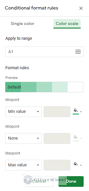
In the Format rules section, you are prompted to choose a gradient of colors to represent your heatmap.
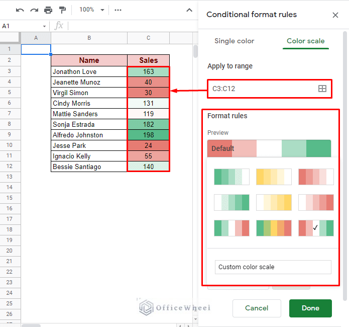
We have chosen the “red to white to green” option, you can choose yours. But if none of the default gradients suit your tastes, you can always customize the Min, Mid, and Max points in the section below.
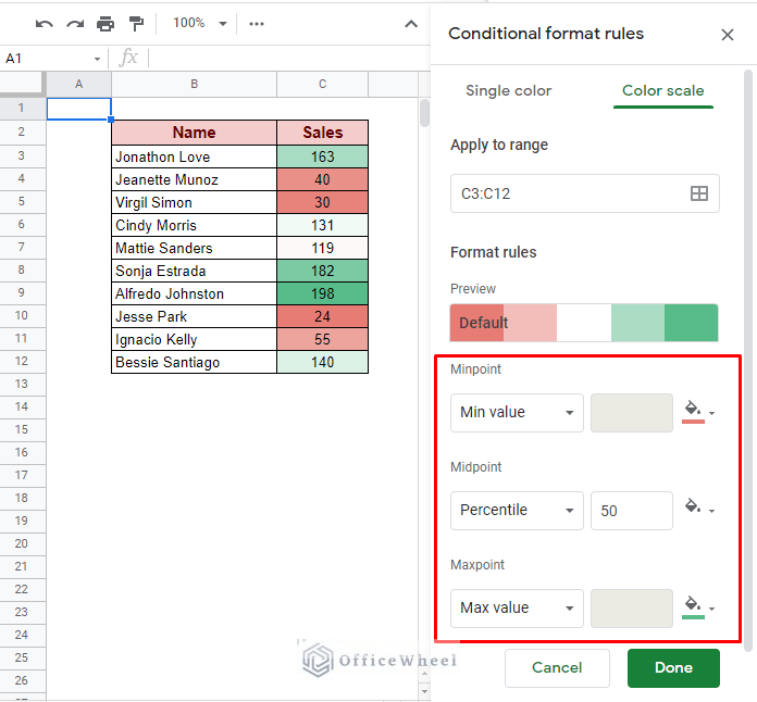
Click Done when you are finished customizing. You have successfully created a heatmap by evaluating the data from your table.
Final Words
Conditional formatting is one of the most used presentation tools in Google Sheets, no matter if the user is a beginner or an expert in the platform. It is also a highly recommended approach to use on complex reports.
We hope that all the processes using conditional formatting in Google Sheets we have discussed in this article help you better understand its potential. Feel free to leave any queries or advice you might have for us in the comments section below.
Related Articles for Reading
- Conditional Formatting with Multiple Conditions Using Custom Formulas in Google Sheets
- Google Sheets: Conditional Formatting with Multiple Conditions
- Change Row Color Based on Cell Value in Google Sheets (4 Ways)
- Google Sheets: Conditional Formatting Row Based on Cell
- Conditional Formatting Based on Another Cell in Google Sheets
- How to Copy Conditional Formatting in Google Sheets