Conditional Formatting with Multiple Conditions Using Custom Formulas in Google Sheets

As complex as custom formulas can be, they are a lifesaver when working with spreadsheets that contain large amounts of data. On the other hand, you have a powerful tool like conditional formatting to help you sift through and highlight important cell values.

In this article, we will be combining these two powerful ideas to apply conditional formatting with multiple conditions using custom formulas in Google Sheets.

Let’s get started.

Custom Formulas for Conditional Formatting with Multiple Conditions

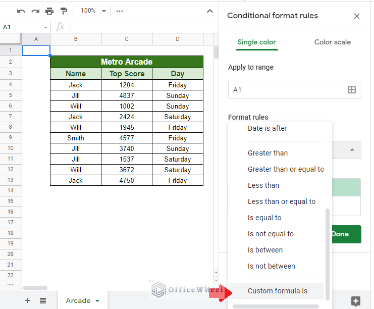
To present our processes, we have created the following worksheet.

It contains three columns of data with varying levels of importance and data types, both text and numbers.

Where do I find the Conditional Formatting menu in Google Sheets?

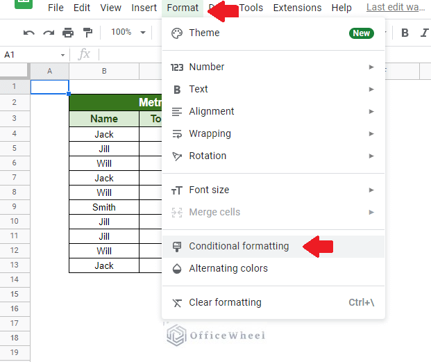
Simply navigate to the Format tab on the top of the window. Here you will find the Conditional formatting option. Clicking on it will open the Conditional format rules menu tray where you can customize the conditional formatting of your worksheet as required.

How do I enter a custom formula for conditional formatting?

Under the Format rules section of the Conditional format rules menu tray, select the drop-down and navigate to the bottom of the list to find the Custom formula is option.

1. Multiple Conditions in a Single Column

For our first method, we will be looking to conditionally format a single column based on the values of the said column.

For this, we will be utilizing some we call the OR logic. It simply means that if one of our multiple conditions is true, a cell will be highlighted.

Thus, for our scenario, we will be highlighting all the cells in the Name column that has the names, Jill or Will.

Step 1: We set our range to the Name column, B4:B13.

Step 2: Apply the custom formula:

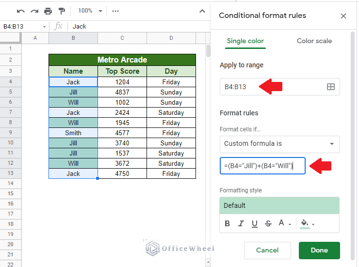
Formula Breakdown:

• We have used simple equals-to (=) operators to determine our condition.
• All text values should be in quotes (“”).
• The plus (+) operator acts as our OR logic to apply two different conditions to our range.
• Our conditions are case-insensitive.

Step 3: Click Done after you are done with any other formatting changes.

Alternative

To further support the OR logic in formulas, Google Sheets provides us with the OR function. It is simply a better way to work on a formula based on OR logic operations.

So, our previous formula transforms to:

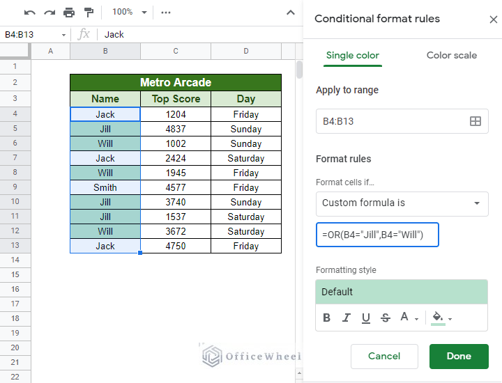
All the separate sections of our conditions, like (B4=”Jill”) and (B4=”Will”), can now be written under one umbrella that is the OR function.

Advanced Customizations

While the formulas we just went through will work just fine in most situations, we can make certain modifications to them to make them more versatile in specific circumstances.

a. Array Values

Our first modification comes with us using an array of values for our conditions. One thing to note is that, unlike Excel, Google Sheets requires us to use the ARRAYFORMULA function when our formula consists of an array of values (usually enclosed in curly braces{}). The function also helps out a range of values, not just one cell.

Thus, our formula becomes:

b. Format Entire Rows

A separate situation may arise where you might have to apply conditional formatting over the entire affected row, not just the cell.

To satisfy this condition, we need to make two changes to our Conditional format rules:

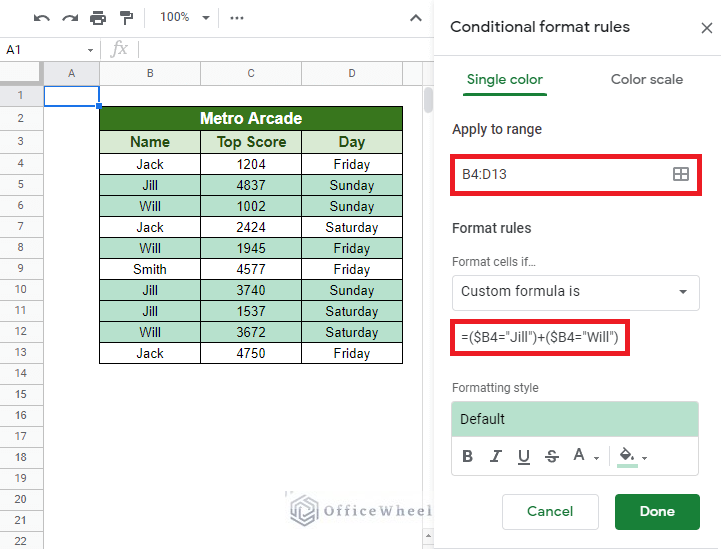
1. Change the range to cover the whole table. In our case, the new range will be B4:D13.
2. Our formula needs some changes as well, namely that of locking the column numbers with absolutes ($). But we keep the row numbers unlocked:
   1. Our first formula: =($B4=”Jill”)+($B4=”Will”)
   2. The second formula: =OR($B4=”Jill”,$B4=”Will”)
   3. The third formula: =ARRAYFORMULA(OR($B4={“Jill”,”Will”}))

To recap, in the OR logic of conditions, any TRUE value will format the cell via conditional formatting.

Reload More: Google Sheets: Conditional Formatting Row Based on Cell

2. Multiple Conditions Based on Value in Multiple Columns

For our next method, we will be following the AND logic of formulas to conditionally format our cells based on multiple conditions.

The AND logic simply means that all of our conditions must be TRUE for the conditional format to highlight our cells.

For our scenario this time, we will be again highlighting the Names that have scored more than 3000 on a Friday.

Step 1: We set our range to the Name column, B4:B13.

Step 2: We apply the custom formula:

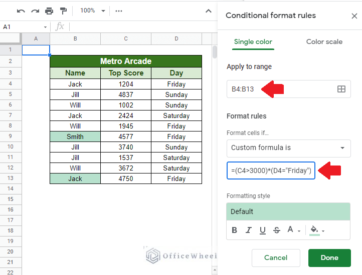
Formula Breakdown:

• We have used simple equals-to (=) operators to determine our condition.
• All text values should be in quotes (“”).
• The multiplication (*) operator acts as our AND logic to apply two different conditions to our range.
• Our conditions are case-insensitive.

Step 3: Click Done after you are done with any other formatting changes.

Alternative

Similar to the OR function, Google Sheets also provides us with the AND function to better utilize formulas with an AND logic.

Thus, our new AND formula will be:

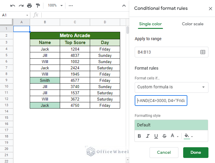
Advanced Customizations

We can perform some of the advanced customizations to our AND logic formula as we have seen for the OR logic.

Entire Rows

Similar changes need to be applied here as well:

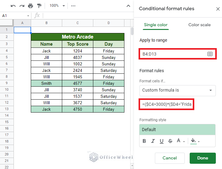
1. We must first change the range of our conditional format to cover the entire table. The new range will be B4:D13.
2. We again have to lock in our column numbers with absolutes ($) to stop the columns from moving with the formula.
   1. Our first formula becomes: =($C4>3000)*($D4=”Friday”)
   2. Our second formula: =AND($C4>3000, $D4=”Friday”)

Note that since no criteria or cell references are common for each condition, we do not need to utilize an array.

Reload More: Conditional Formatting with Multiple Conditions Using Custom Formulas in Google Sheets

Similar Readings

• How to Search in All Sheets in Google Sheets (An Easy Guide)
• Google Sheets: Highlight Row If Cell Is Empty
• How to Highlight Duplicates for Multiple Columns in Google Sheets
• Conditional Formatting with Checkbox in Google Sheets
• How to Copy Conditional Formatting in Google Sheets

3. Combining AND and OR Conditions

For our final scenario, we will be combining some conditions from both of our previous scenarios.

This time, we want to highlight the entire row where Jack and Jill have scored more than 3000 points. For advanced conditions like these, built-in functions won’t cut it. For that, we need to create our very own custom formula.

We begin with our OR conditions. We need the scores of either Jack or Jill. Our formula:

We need to highlight the entire row, so we need to lock our columns:

The condition where we calculate the score:

Combining both of our conditions so that both of them have to return TRUE:

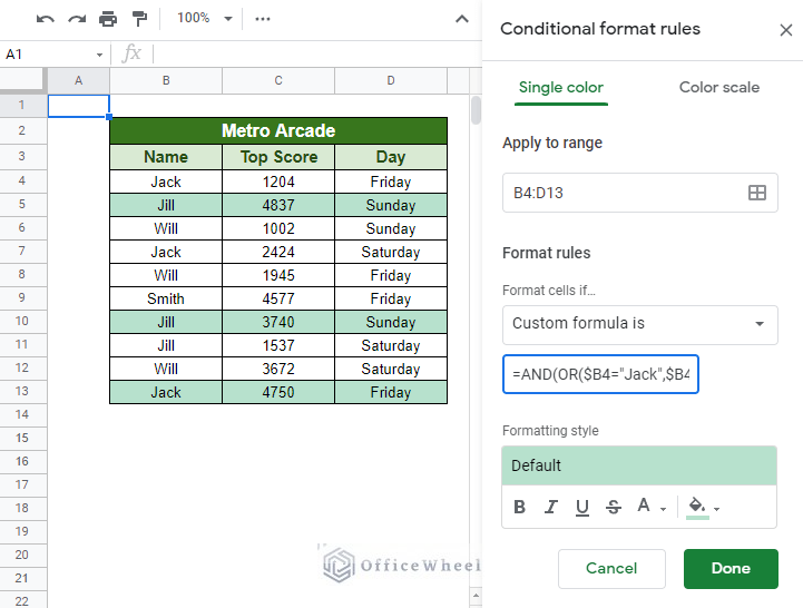
Reload More: Using Conditional Formatting With Custom Formula in Google Sheets

Final Words

Conditional formatting is perhaps one of the more powerful tools in Google Sheets with near-endless applications, especially with custom formulas. We hope that through this article, you will now be able to apply conditional formatting with a custom formula based on multiple conditions in Google Sheets.

Feel free to comment on any queries or advice you might have for us in the comments section.

Related Articles

• Conditional Formatting Based on Another Cell in Google Sheets
• Change Row Color Based on Cell Value in Google Sheets (4 Ways)
• Match Multiple Values in Google Sheets (An Easy Guide)
• Google Sheets: Conditional Formatting with Multiple Conditions
• How to Use VLOOKUP for Conditional Formatting in Google Sheets
• Use Multiple IF Statements in Google Sheets (5 Examples)
• How to Use AND Function in Google Sheets (4 Useful Examples)