When we use a function within another function, it is called a nested function. The privilege of using nested functions in Google Sheets and Excel makes them very dependable for various calculations. This article will discuss how you can use the nested IF function in Google Sheets. The IF function is one of the most popular functions in Google Sheets. Here, we will use multiple IF functions along with the AND and OR functions. Also, we’ll discuss several alternatives to the nested IF function.
A Sample of Practice Spreadsheet
You can copy our practice spreadsheets by clicking on the following link. The spreadsheet contains an overview of the datasheet and an outline of the described ways to use the nested IF function.
4 Helpful Ways to Use Nested IF Function in Google Sheets
In this section, we’ll show you 4 helpful ways to use the nested IF function in Google Sheets. We will also use the OR and AND functions along with multiple IF functions.
1. Using Multiple IF Functions
First, let’s create nested IF functions only using multiple IF functions. For that, we will demonstrate the following two examples.
1.1 Calculating Students’ Final Grade
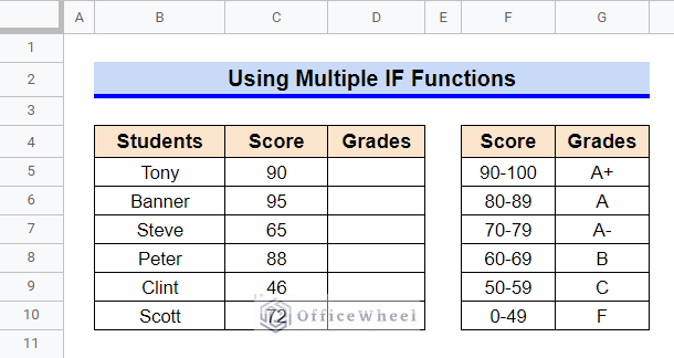
In this example, we will calculate grades for several students of a class based on their marks, using the nested IF function.
Steps:
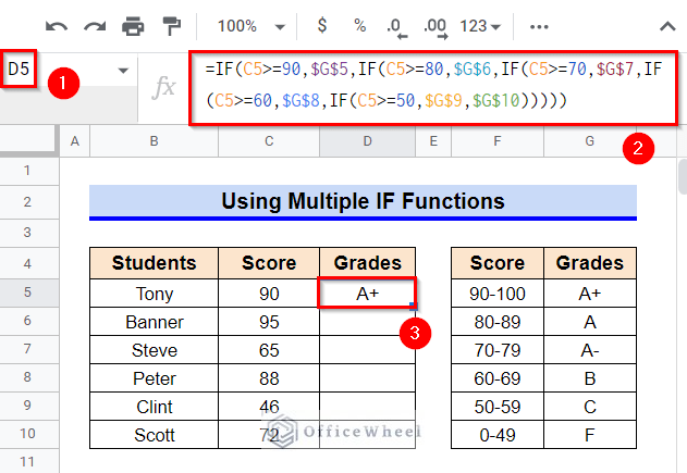
- First, select Cell D5.
- After that, type in the following formula-
=IF(C5>=90,$G$5,IF(C5>=80,$G$6,IF(C5>=70,$G$7,IF(C5>=60,$G$8,IF(C5>=50,$G$9,$G$10)))))- Finally, press Enter key to get the required Grade.
Formula Breakdown
- IF(C5>=90,$G$5,IF(C5>=80,$G$6,IF(C5>=70,$G$7,IF(C5>=60,$G$8,IF(C5>=50,$G$9,$G$10)))))
The first IF function checks whether the score in Cell C5 is greater than or equal to 90. If the logical test is True then it returns the content of Cell G5. Else, it moves on to the next IF function. The same process goes on for other IF functions as well.
- Now, hover your mouse pointer above the bottom right corner of the selected cell.
- The Fill Handle icon will be visible. Use this icon to copy the formula to other cells.
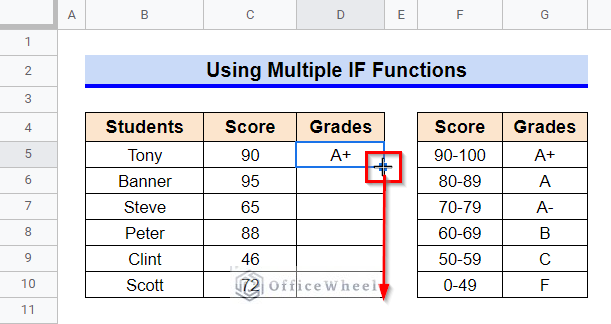
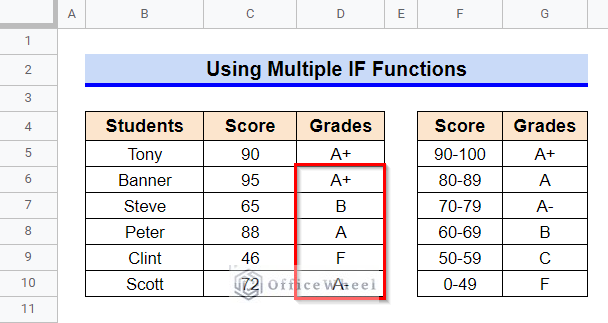
- Thus, you can calculate grades using the nested IF function.
Read More: How to Use IF Function in Google Sheets (6 Suitable Examples)
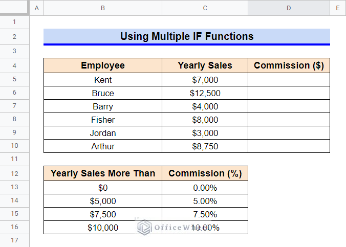
1.2 Estimating Sales Commission
Now, for another example, we’ll estimate yearly sales commissions received by employees of a company using the nested IF function.
Steps:
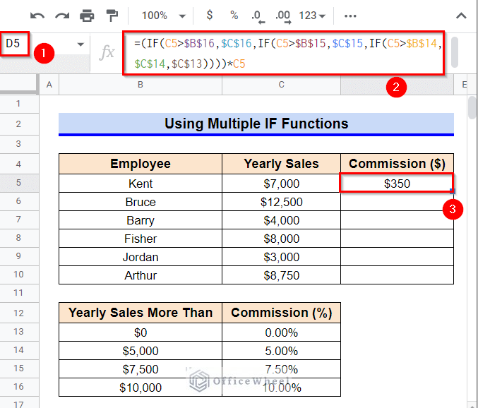
- Select Cell D5 first.
- Afterward, type in the following formula-
=(IF(C5>$B$16,$C$16,IF(C5>$B$15,$C$15,IF(C5>$B$14,$C$14,$C$13))))*C5- Then, press Enter key to get the required amount of commission value.
Formula Breakdown
- (IF(C5>$B$16,$C$16,IF(C5>$B$15,$C$15,IF(C5>$B$14,$C$14,$C$13))))*C5
The first IF function runs the logical test of whether the value in Cell C5 is greater than the value in Cell B16. If the logical test is True then it returns the content of Cell C16. Else, it moves on to the next IF function. A similar process goes on for the remaining IF functions too. The returned value by the nested IF function is finally multiplied by the value in Cell C5 to estimate the commission amount.
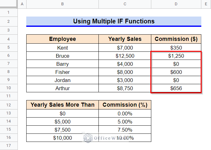
- Finally, use the Fill Handle icon to copy the formula to other cells as well.
Read More: How to Use Multiple IF Statements in Google Sheets (5 Examples)
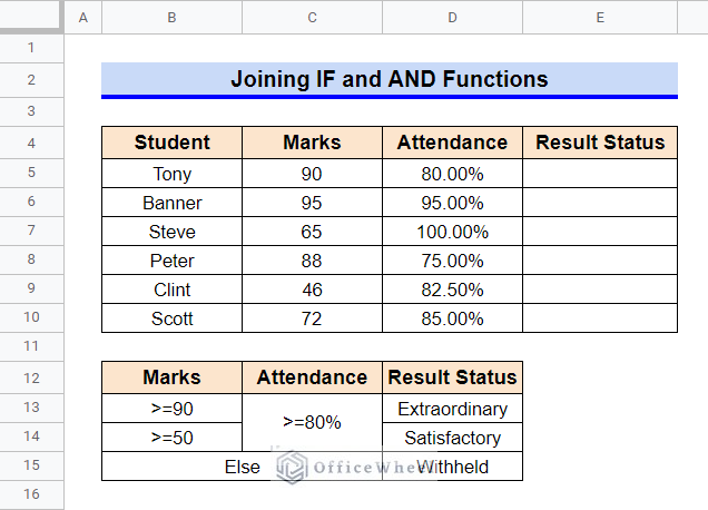
2. Joining IF and AND Functions
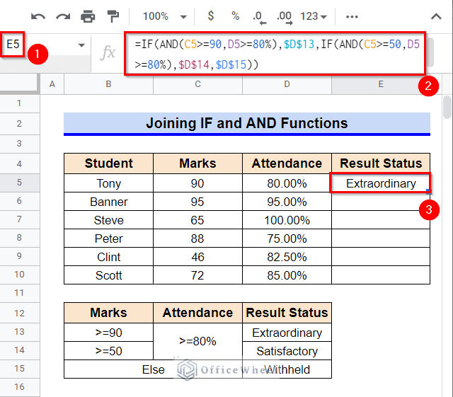
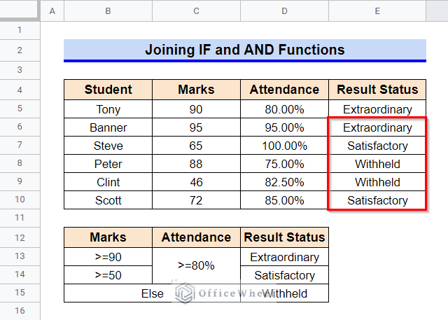
We can combine the AND function with multiple IF functions to form a nested statement that will calculate values based on mutually inclusive dependent conditions. We will assess students’ result status based on their marks and attendance.
Steps:
- To start, select Cell E5 and then type in the following formula-
=IF(AND(C5>=90,D5>=80%),$D$13,IF(AND(C5>=50,D5>=80%),$D$14,$D$15))- Now, press the Enter key to get the required status.
Formula Breakdown
- AND(C5>=90,D5>=80%)
This AND function checks whether both the given criteria are true or not. It returns True if both the criteria are true. Else, it returns False.
- IF(AND(C5>=90,D5>=80%),$D$13,IF(AND(C5>=50,D5>=80%),$D$14,$D$15))
If the logical test performed by using the first AND function is True, then the first IF function returns the value in Cell D13. Else, it moves on to the second IF function. The second IF function works similarly to the first one. It returns the value in Cell D14 if the logical test is true. Else, it returns the value in Cell D15.
- Finally, use the Fill Handle icon to copy the formula in other cells as well.
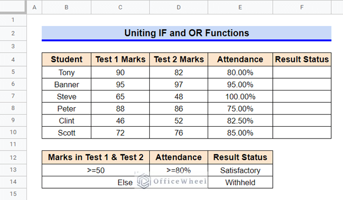
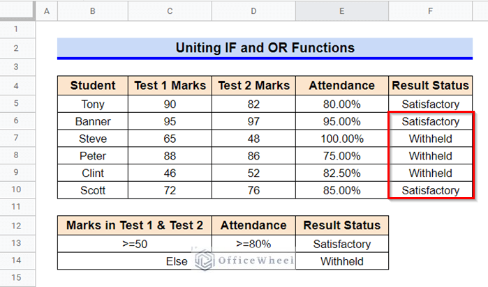
3. Uniting IF and OR Functions
Executing this method is very similar to the previous example, except the criteria used in this method will be mutually exclusive. We’ll enumerate students’ result status based on attendance and marks from two tests this time.
Steps:
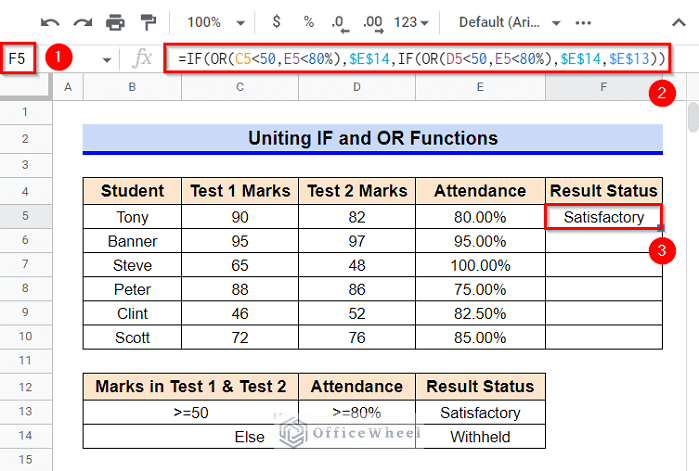
- First, select Cell F5.
- Then, type in the following formula-
=IF(OR(C5<50,E5<80%),$E$14,IF(OR(D5<50,E5<80%),$E$14,$E$13))- Afterward, press the Enter key to get the required result.
Formula Breakdown
- OR(C5<50,E5<80%)
This OR function checks whether any of the given criteria is true or not. It returns True if any of the criteria is true. Else, it returns False.
- IF(OR(C5<50,E5<80%),$E$14,IF(OR(D5<50,E5<80%),$E$14,$E$13))
If the logical test performed by using the first OR function is True, then the first IF function returns the value in Cell E14. Else, it moves on to the second IF function. The second IF function works similarly to the first one. It returns the value in Cell E14 if the logical test is true. Else, it returns the value in Cell E15.
- Finally, use the Fill Handle icon to copy the formula in other cells too.
Read More: How to Use IF and OR Formula in Google Sheets (2 Examples)
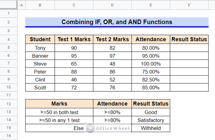
4. Combining IF, OR, and AND Functions
The OR and AND functions can be combined with multiple IF functions in a single nested function. For this method, we’ll enumerate students’ result statuses based on marks in two tests and their attendance. If a student gets more than 50 marks on both tests and has an attendance of 80% or more, his result status will be “Good”. On the other hand, if a student gets 50 or more marks in only one test and has an attendance of 80% or more, his result status will be “Satisfactory”. Students with any other category will have a “Withheld” status.
Steps:
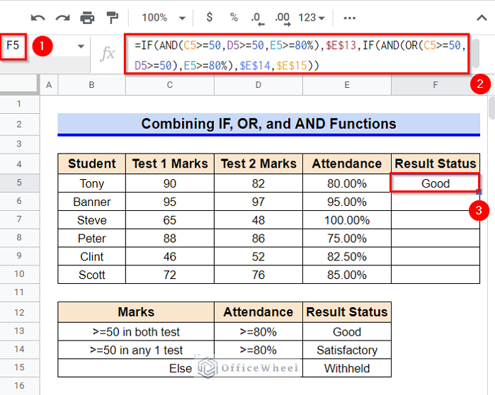
- To start, select Cell F5 first.
- Afterward, type in the following formula-
=IF(AND(C5>=50,D5>=50,E5>=80%),$E$13,IF(AND(OR(C5>=50,D5>=50),E5>=80%),$E$14,$E$15))- Finally, press Enter key to get the required result.
Formula Breakdown
- OR(C5>=50,D5>=50)
This OR function checks whether any of the given criteria is true or not. It returns True if any of the criteria is true. Else, it returns False.
- AND(OR(C5>=50,D5>=50),E5>=80%)
This AND function returns True if the OR function returns True and the other criterion E5>=80% is also true. Else, it returns False.
- IF(AND(C5>=50,D5>=50,E5>=80%),$E$13,IF(AND(OR(C5>=50,D5>=50),E5>=80%),$E$14,$E$15))
The first IF function returns the value in Cell E13 if the logical test performed using the AND function is true. Else, it moves on to the second IF function, which works similarly. If both the IF function logical tests are false then value in Cell E15 is returned.
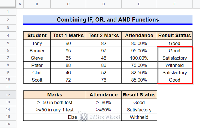
- Now, use the Fill Handle icon to copy the formula in the other cells of Column F.
Alternatives to Nested IF Function in Google Sheets
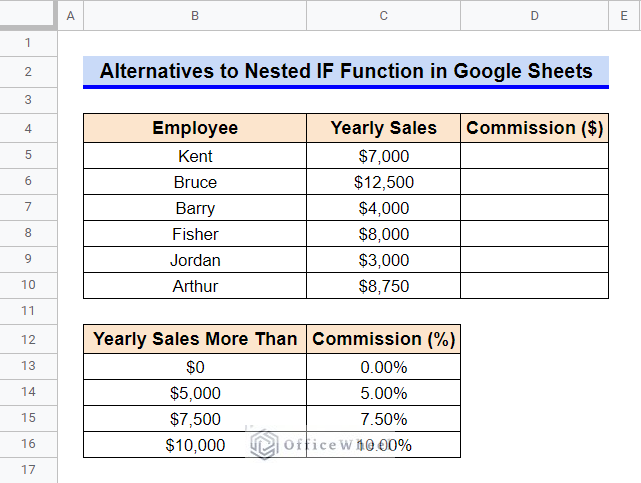
There are a few alternatives to the nested IF function in Google Sheets. Here, we’ll discuss 3 alternatives that are much simpler to use compared to the nested IF function. We’ll use these functions to calculate yearly sales commissions from the following dataset. The required result was previously calculated using the nested IF function in Example 1.2 of the first method in the previous section.
Read More: How to Use Nested IF Statements in Google Sheets (3 Examples)
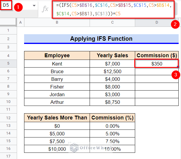
1. Applying IFS Function
The nested IF function is usually employed to incorporate multiple conditions and subsequent values. The IFS function can be used as an alternative in such scenarios.
Steps:
- First, select Cell D5.
- Afterward, type in the following formula-
=(IFS(C5>$B$16,$C$16,C5>$B$15,$C$15,C5>$B$14,$C$14,C5>$B$13,$C$13))*C5- Now, press Enter key to get the required value.
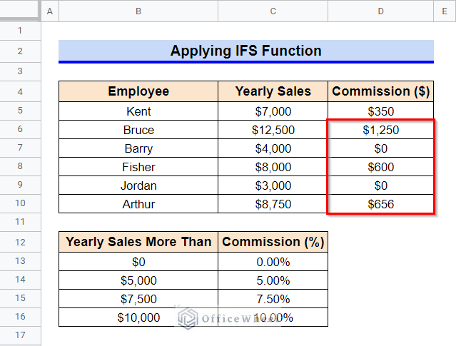
- Finally, use the Fill Handle icon to copy the formula to other cells.
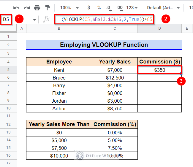
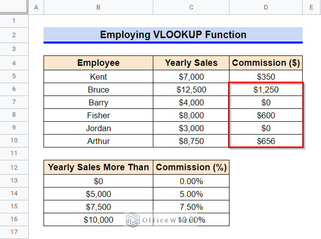
2. Employing VLOOKUP Function
Another alternative to the nested IF function is the VLOOKUP function which can search through a range for any search key. Although, one must remember that the search key has to be in the first column of the provided range.
Steps:
- To start with, select Cell D5.
- Then, type in the following formula-
=(VLOOKUP(C5,$B$13:$C$16,2,True))*C5- Finally, press Enter key to get the required value.
- use the Fill Handle icon to copy the formula to other cells.
Read More: How to Use VLOOKUP for Conditional Formatting in Google Sheets
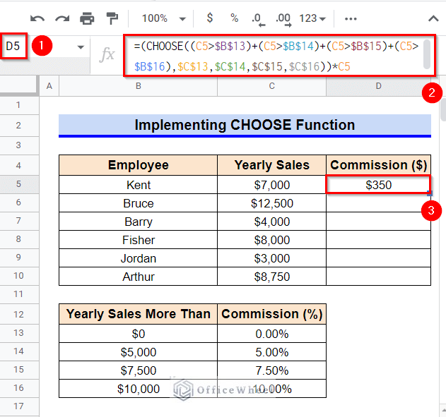
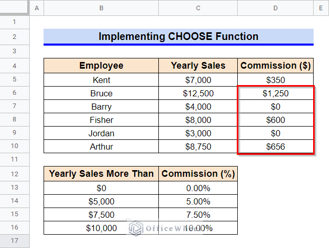
3. Implementing CHOOSE Function
We can also use the CHOOSE function as an alternative to the nested IF function. The CHOOSE function can return an element from a list of choices.
Step:
- In the beginning, select Cell D5.
- Afterward, type in the following formula-
=(CHOOSE((C5>$B$13)+(C5>$B$14)+(C5>$B$15)+(C5>$B$16),$C$13,$C$14,$C$15,$C$16))*C5- Now, press Enter key to get the required result.
- In the end, use the Fill Handle icon to copy the formula to other cells of Column D.
Things to Be Considered
- There are no false statements in the arguments of the IFS function.
- The search key has to be in the first column of the range while using the VLOOKUP function.
Conclusion
This concludes our article on how to use the nested IF function in Google Sheets. I hope the article was sufficient for your requirements. Feel free to leave your thoughts on the article in the comment section. Visit our website OfficeWheel.com for more helpful articles.
Related Articles
- Google Sheets IF Statement in Conditional Formatting
- How to Do IF THEN in Google Sheets (3 Ideal Examples)
- Highlight Cell If Value Exists in Another Column in Google Sheets
- How to Use IF Condition Between Two Numbers in Google Sheets
- Conditional Formatting with Multiple Conditions Using Custom Formulas in Google Sheets
- Google Sheets: Conditional Formatting with Multiple Conditions