The IF and OR functions are 2 logical operators in Google Sheets. The IF function gives TRUE when all the logic is TRUE otherwise FALSE. Moreover, the OR function gives TRUE when either of the values is TRUE and FALSE when all the values are FALSE. So, we can combine these 2 functions to get our desired output by setting up multiple criteria. In this article, I’ll show 2 suitable examples to use the IF and OR formula in Google Sheets with clear images and steps.
A Sample of Practice Spreadsheet
You can download Google Sheets from here and practice very quickly.
2 Suitable Examples to Use IF and OR Formula in Google Sheets
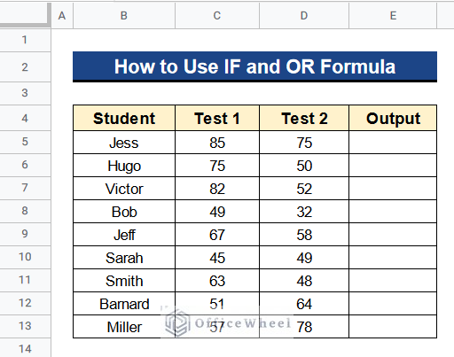
Let’s get introduces to our dataset first. Here we have some students in Column B, their test 1 scores in Column C, and their test 2 scores in Column D. The pass mark for any of the tests is 51. We want the output as “Pass” if a student gets at least 51 marks in any of the 2 tests otherwise “Fail”. So now we’ll see 2 suitable examples to use the IF and OR formula in Google Sheets with multiple conditions. Let’s see the examples below.
Example 1. Combining IF and OR Functions
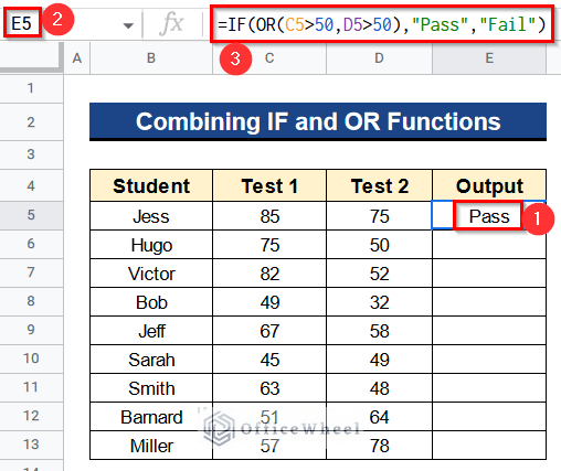
We can combine the IF and OR functions in Google Sheets to logically get some output. Here we have 2 test scores and we’ll get our output as “Pass” if a student gets above 50 on either of the 2 tests. Or he’ll get a “Fail”.
Steps:
- Firstly, type the following formula in Cell E5–
=IF(OR(C5>50,D5>50),"Pass","Fail")- Secondly, hit Enter to get the result quickly.
Formula Breakdown
- OR(C5>50,D5>50)
At first, this function returns TRUE if any of the values from Cell C5 and D5 is greater than 50 otherwise it returns FALSE.
- IF(OR(C5>50,D5>50),”Pass”,”Fail”)
At last, the IF function gives the output as “Pass” if the conditions are TRUE. Or it’ll give the output as “Fail”.

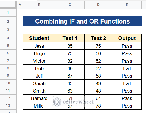
- Next, you’ll get the outputs in Column E.
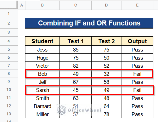
- Finally, you’ll see that only 2 students get a “Fail” in Row 8 and 10 because they couldn’t match the 2 criteria. They get less than 51 on both tests.
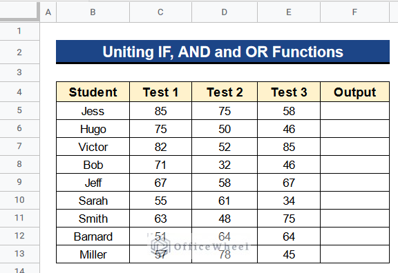
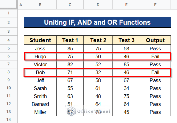
Example 2. Uniting IF, AND and OR Functions
The AND function is also a logical operator in Google Sheets. It gives TRUE when all the values are TRUE. When any of the values is FALSE then it gives FALSE. That’s why we can unite this function with the IF and OR functions and apply them in Google Sheets as an alternative to nested IF functions for multiple criteria. Like in this case we have the following dataset having 3 tests no in Columns C, D, and E. Now, we want our output as “Pass” if a student gets at least 51 marks in any of the 2 tests out of the 3 tests. Or the output will be “Fail”. Let’s see how to do it.
Steps:
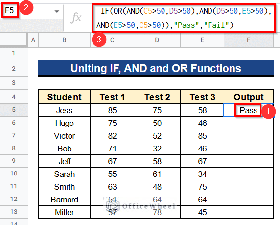
- First of all, write the following formula in Cell F5–
=IF(OR(AND(C5>50,D5>50),AND(D5>50,E5>50),AND(E5>50,C5>50)),"Pass","Fail")- After that, press Enter to get the output.
Formula Breakdown
- AND(C5>50,D5>50)
Before all, the AND function returns TRUE if the values from Cell C5 and D5, both are greater than 50. If any of the 2 values are not greater than 50 then it will return FALSE.
- AND(D5>50,E5>50)
Consequently, this function gives the same output as the previous one. But it works for Cell D5 and E5.
- AND(E5>50,C5>50)
Again, this also does the same task for Cell E5 and C5.
- OR(AND(C5>50,D5>50),AND(D5>50,E5>50),AND(E5>50,C5>50))
Moreover, the OR function gives TRUE when any of the 3 conditions match otherwise FALSE.
- IF(OR(AND(C5>50,D5>50),AND(D5>50,E5>50),AND(E5>50,C5>50)),”Pass”,”Fail”)
Finally, this function returns the output as “Pass” if the conditions are TRUE. Or it’ll return the output as “Fail”.
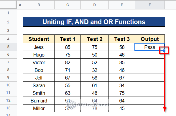
- Then, use the Fill Handle tool to apply the formula to the rest of the cells of Column F.
- Afterward, we’ll get our desired output in Column F.
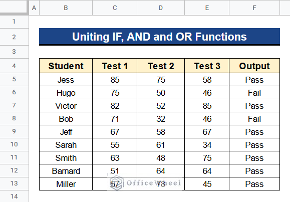
- Ultimately, you’ll find that only 2 students get a “Fail” in Rows 6 and 8. It is because they couldn’t match the 3 criteria. They get less than 51 on the 2 tests out of the 3 tests. The rest of the students match the 3 criteria and get a “Pass”.
Things to Remember
- You have to apply the Fill Handle tool to use the formula in all of the cells. You can’t use the ARRAYFORMULA function in this case. Because it is a limitation of Google Sheets that you can’t combine the ARRAYFORMULA function with the OR and AND functions in Google Sheets.
Conclusion
That’s all for now. Thank you for reading this article. In this article, I have discussed 2 suitable examples to use the IF and OR formula in Google Sheets. Please comment in the comment section if you have any queries about this article. You will also find different articles related to google sheets on our officewheel.com. Visit the site and explore more.
Related Articles
- Google Sheets IF Statement in Conditional Formatting
- How to Do IF THEN in Google Sheets (3 Ideal Examples)
- How to Use the Find Function in Google Sheets (An Easy Guide)
- Google Sheets: Conditional Formatting with Multiple Conditions
- Highlight Cell If Value Exists in Another Column in Google Sheets
- How to Use IF Condition Between Two Numbers in Google Sheets