The REGEXMATCH function in Google Sheets determines whether a text string fits a regular expression. If it does, the function returns TRUE; otherwise, it returns FALSE. We can use the REGEXMATCH function to match multiple values across the dataset. In this article, I will demonstrate 3 easy ways to match multiple values using the REGEXMATCH function in Google Sheets .
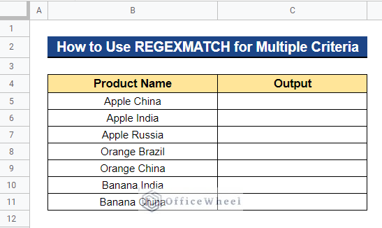
3 Easy Ways to Use REGEXMATCH Function for Multiple Criteria in Google Sheets
We will use the dataset below to demonstrate the examples of matching multiple values using the REGEXMATCH function in Google Sheets. The dataset contains the Product Name and we want to match multiple values across this column.
1. Using REGEXMATCH Function Only
The REGEXMATCH function in Google Sheets may be used to match multiple values throughout the dataset. Multiple values inside a column or even multiple values within a cell string can be matched using the REGEXMATCH function.
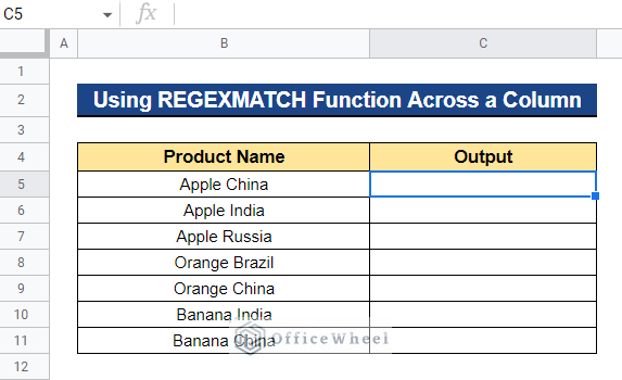
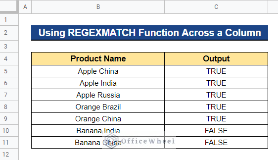
1.1 Across a Column
The REGEXMATCH function in Google Sheets allows us to match multiple values inside a column. Assume that we want to determine whether cells in the column of our dataset include the words Apple or Orange.
Steps:
- First, select a cell where you want to apply the formula. In our case, we selected Cell C5.
- Now, type the formula below and press Enter–
=REGEXMATCH(B5,"Apple|Orange")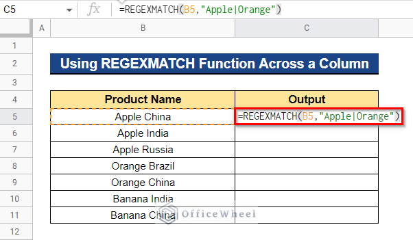
- As a result, it will return TRUE if the cell contains the word Apple or Orange. Otherwise, it will return FALSE. Now drag the Fill Handle icon downward to apply the formula to the remaining cells.
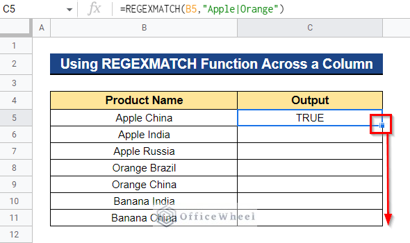
- Thus, all the cells that contain the word Apple or Orange will return the value TRUE.
Read More: How to Make REGEXMATCH Case Insensitive in Google Sheets
1.2 Across a Cell
Using Google Sheets’ REGEXMATCH function, we can match multiple values in a single cell. In our dataset, let’s imagine that we want to see which cells in the column contain Apple at the start and India at the end. When you wish to match the first and last word from the cell content, use this method.
Steps:
- Choose the cell to which you wish to apply the formula first. In our case, we chose Cell C5. Now, enter the following formula and hit Enter–
=REGEXMATCH(B5,"^Apple[a-zA-Z ]+India$")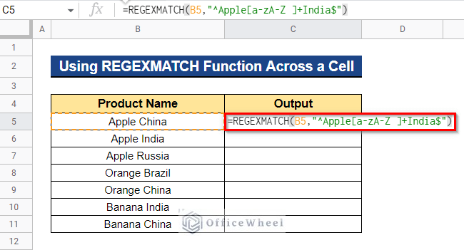
- In this case, we use the wedge sign (^) before Apple to check if Cell C5 begins with Apple and the dollar symbol ($) after India to check whether Cell C5 finishes with India. Between the words Apple and India, we inserted the symbol [a-zA-Z]+ to represent any combination of lower- and upper-case alphabets. As you can see, there is a space after the letter Z because we want to allow spaces in the sequence.
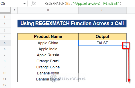
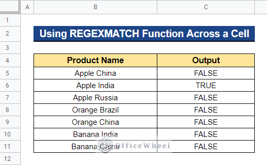
- Therefore, if the words Apple and India are present in the cell, it will return TRUE. If not, FALSE will be returned. To apply the formula to the remaining cells, drag the Fill Handle icon downward.
- Thus, all the cells that contain both the word Apple and India, will return the value TRUE.
Read More: If Cell Contains Text Then Return Value in Another Cell in Google Sheets
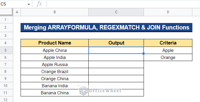
2. Merging ARRAYFORMULA, REGEXMATCH & JOIN Functions
To match multiple values across a column in Google Sheets based on a list, we may combine the ARRAYFORMULA, REGEXMATCH, and JOIN functions. And we have the list in Column D.
Steps:
- Select the cell to which you want to apply the formula first. In our scenario, we selected Cell C5.
- Now, input the subsequent formula and press Enter–
=ARRAYFORMULA(REGEXMATCH(B5,JOIN("|",$D$5:$D$6)))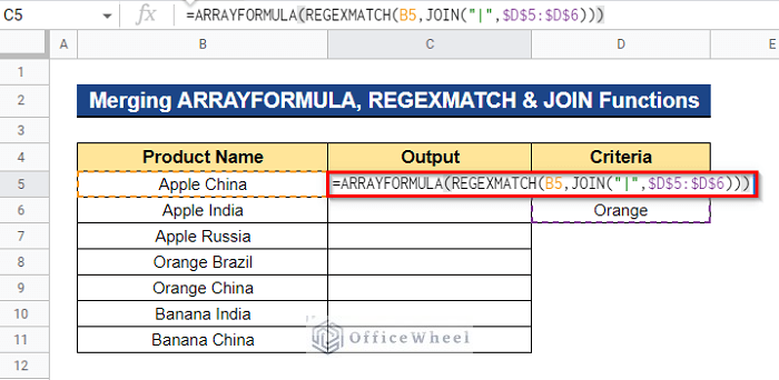
Formula Breakdown
- JOIN(“|”,$D$5:$D$6)
First, the JOIN function will concatenate the items of one or many one-dimensional arrays utilizing a defined delimiter.
- REGEXMATCH(B5,JOIN(“|”,$D$5:$D$6))
Then, the REGEXMATCH function will determine whether the text string matches the cell references.
- ARRAYFORMULA(REGEXMATCH(B5,JOIN(“|”,$D$5:$D$6)))
Here, the ARRAYFORMULA function conducts several computations on a single array item.
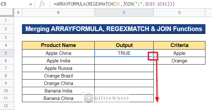
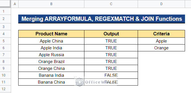
- As a consequence, if the cell includes the term that is provided in the Criteria column, it will return TRUE. If not, FALSE will be returned. To apply the formula to the remaining cells, drag the Fill Handle symbol downward.
- All of the cells that contain the term listed in the Criteria column will thus return the result TRUE.
Read More: How to Use ARRAYFORMULA with IF Function in Google Sheets
3. Combining REGEXMATCH & AND Functions
We may match multiple values in a cell string by using the REGEXMATCH and AND functions. When employing this technique, you don’t have to be concerned about excess character or space.
Steps:
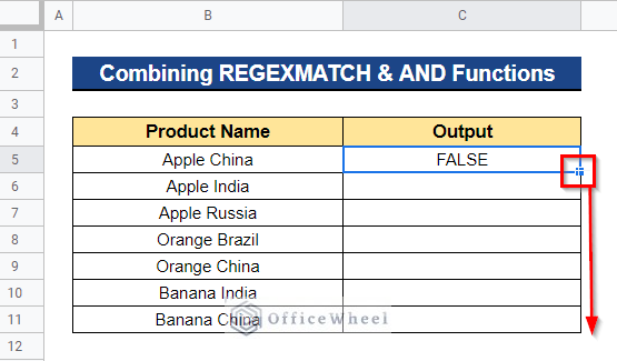
- First, decide which cell you want the formula to be applied to. In our instance, we selected Cell C5. Now, input the formula below and press Enter–
=AND(REGEXMATCH(B5,"Apple"),AND(REGEXMATCH(B5,"India")))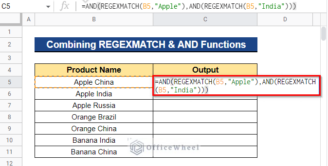
Formula Breakdown
- REGEXMATCH(B5,”Apple”)
First, the REGEXMATCH function will determine when the text string matches the cell references.
- AND(REGEXMATCH(B5,”Apple”),AND(REGEXMATCH(B5,”India”)))
If all of the supplied arguments are logically true, the AND function will then return TRUE; but, if any of the supplied arguments are logically untrue, it will return FALSE.
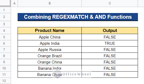
- Therefore, the cell will return TRUE if the terms Apple and India are present. FALSE will be returned if not. Dragging the Fill Handle symbol downward will apply the formula to the remaining cells.
- Thus, you will get the desired output.
Conclusion
In this article, I have shown how to match multiple values across a cell or a column using the REGEXMATCH function in Google Sheets. I hope this will be helpful. Please feel free to ask any quarries or comment on any ideas in the comment section below. To explore more, visit Officewheel.com.
Related Articles
- Highlight Row Based on Date in Google Sheets (2 Suitable Ways)
- How to Highlight Row If Cell Is Not Empty in Google Sheets
- Find if Date is Between Dates in Google Sheets (An Easy Guide)
- How to Use Multiple IF Statements in Google Sheets (5 Examples)
- Conditional Formatting with Multiple Conditions Using Custom Formulas in Google Sheets
- Google Sheets: Conditional Formatting with Multiple Conditions