Highlight Duplicates in Google Sheets (4 Ways)

The ability to highlight duplicates in any worksheet is crucial for a variety of reasons. While it may sound easy to do, it can prove to be very complex if you do not understand how Google Sheets perceives your data.

Once we understand that, we can use the only tool, Conditional Formatting, to highlight duplicates in Google Sheets.

Note that, the Conditional Formatting tool of Google Sheets is not only used for formatting data but also dynamic highlighting according to criteria. Meaning, if any of your data changes within the format range, the tool will also change accordingly.

With that, let’s get started.

4 Ways to Highlight Duplicates in Google Sheets

1. Highlight All Duplicate Instances in Google Sheets

The Formula for Finding Duplicates

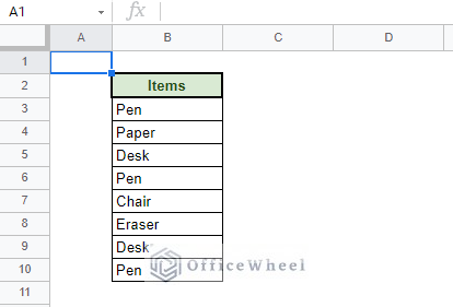
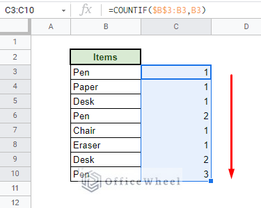
Let’s start by understanding how Google Sheets recognizes duplicates within a certain selected range. As we can see, the following list of Items contains certain duplicates.

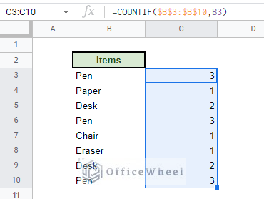
By doing a simple count, we can quantify the number of duplicates of each item, we use the COUNTIF function to do that. And our formula is:

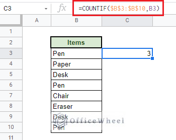
This formula helps to count the number of duplicates within the given range (covered by absolutes ($)) and checks for the condition referenced in cell B3 in our case.

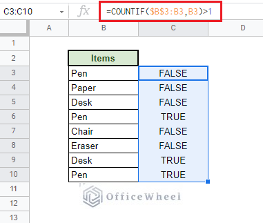
Conditional Formatting in Google Sheets will be checking whether an item/value occurs more than once within the given range. Thus we also have to add the condition “>1” to our formula to find whether the item is a duplicate or not as a Boolean.

Thus, our new formula is:

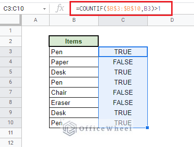
Applying the Formula to Conditional Formatting

Now that we have found our formula, it is time to apply it to Conditional Formatting.

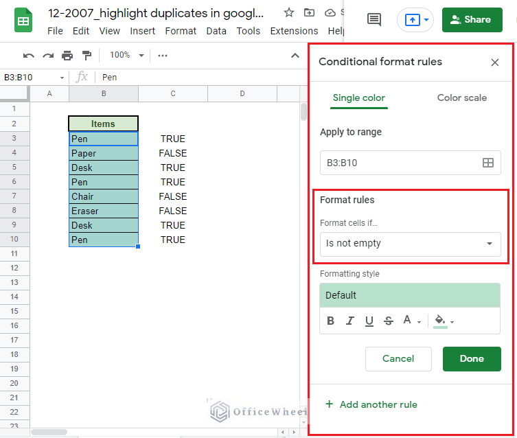
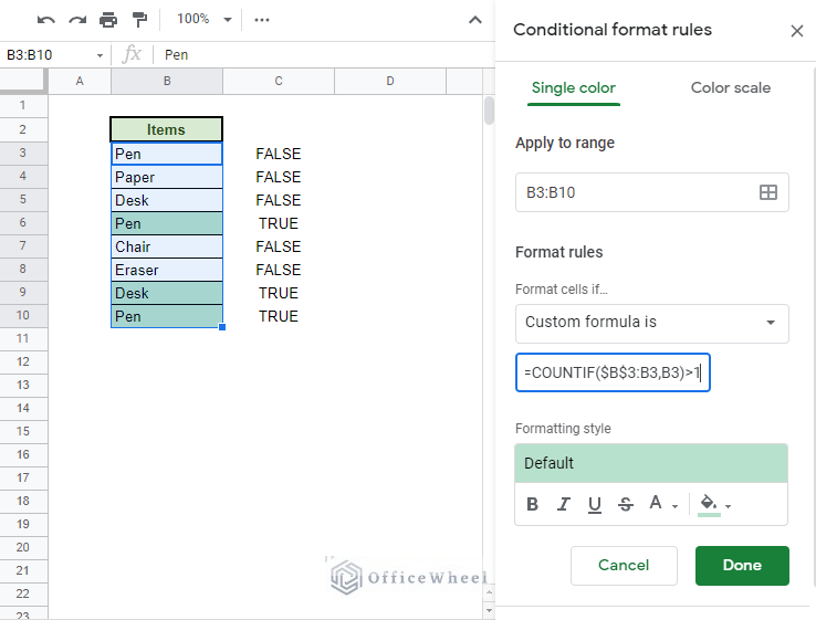
Step 1: Select the range (B3:B10 for us) and open the Conditional Formatting menu. Format tab > Conditional formatting

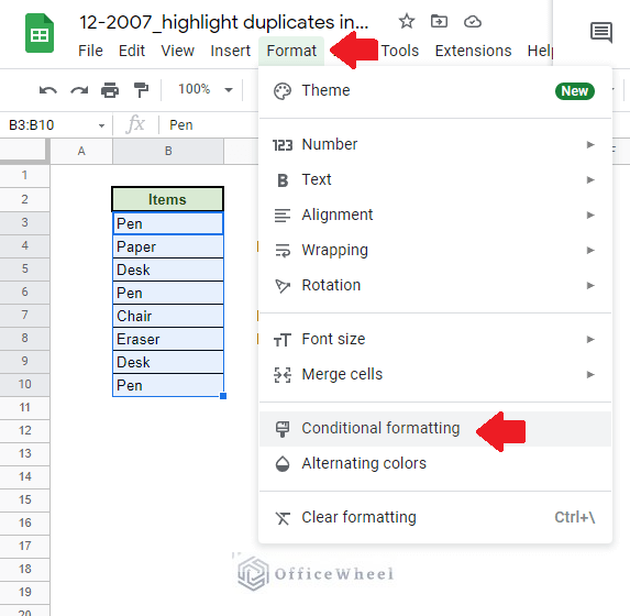
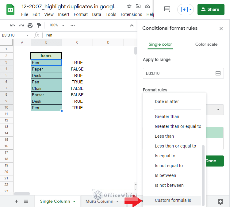
Step 2: Choose the Custom formula is option under the Format rules section.

Step 3: Apply the formula =COUNTIF($B$3:$B$10,B3)>1. You can choose the type of highlight that you want from the Formatting style section.

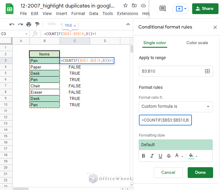
Step 4: Click Done.

This method highlights ALL the duplicates with a range. We also call this finding duplicates including the 1st occurrence.

2. Highlight Duplicates in Multiple Columns in Google Sheets

Let’s now move on to multiple columns worth of data from single columns to further show off the capabilities of Google Sheets’ Conditional Formatting.

We will be using the same foundation formula that we used in the last method. But since our range now has multiple columns, we need to apply some modifications to our formula.

To begin with, open the Conditional formatting rules menu tray as before (Format tab > Conditional formatting). Select the Custom formula is option.

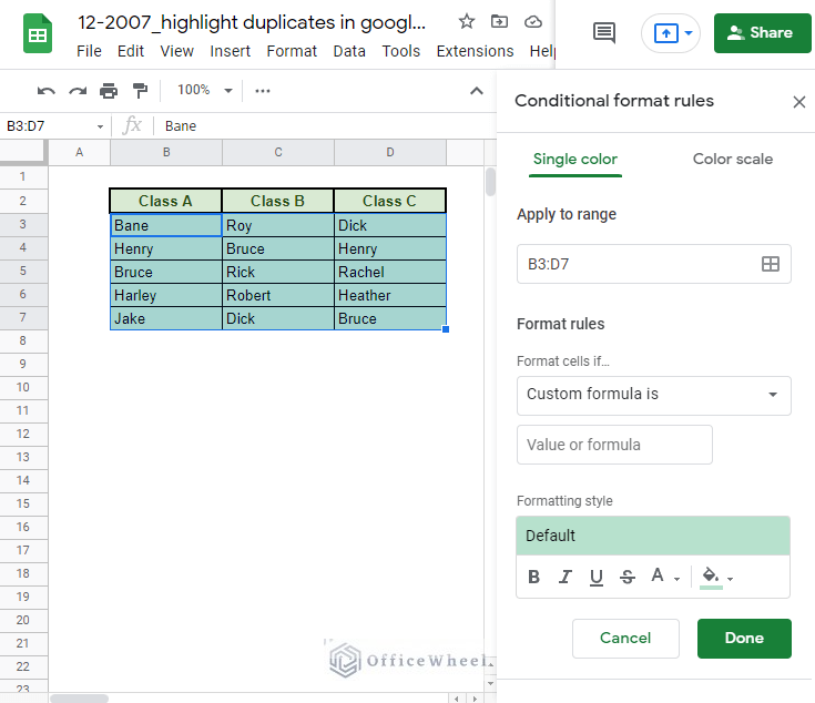
We will be changing our selected range from B3:B10 to B3:D7 accordingly and applying absolutes ($) to this range. So, our new formula is:

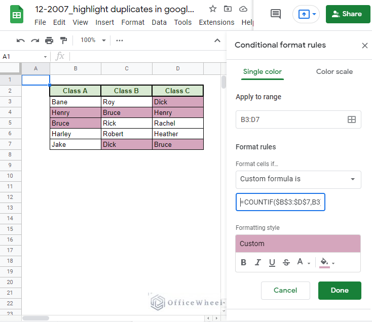
We have changed some highlight formatting, but the principles remain the same.

We have successfully highlighted all the duplicates in the given columns in Google Sheets.

3. Highlight Duplicates without the First Occurrence (Duplicate Instance Only)

Till now, we have included the first occurrence of duplicate values in our highlights. But what if you wanted to show only the duplicate occurrences excluding the first value?

We will show you how to do that in this section.

Creating the Formula

Let’s go back to our dataset used in method 1.

We are still going to be using the COUNTIF function, but the change comes with the range that we are going to be inputting.

Our new range in the COUNTIF function is $B$3:B3. The second portion will increment as we go down the rows.

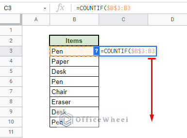
Our criterion will the same as before, B3.

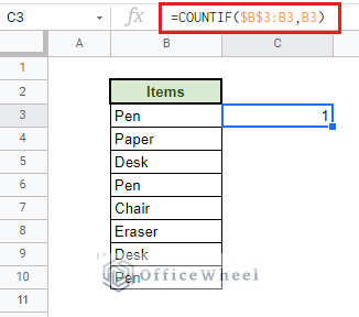
Previously we had counted all of the occurrences of the criterion at once, thus we saw all of the numbers of occurrences from the beginning. This new formula will count the duplicates incrementally as we go down the rows, as we can see here:

For the final touches, we will add a Boolean condition for the Conditional Formatting.

So our final version of the formula is:

Applying the Conditional Formatting

Now that we have the final version of the formula, we can move forward to applying it to highlight the duplicate instances in our Item list.

Step 1: Select the range and open the Conditional formatting rules menu tray. Format tab> Conditional formatting

Step 2: Apply the custom formula: =COUNTIF($B$3:B3,B3)>1

Step 3: Click Done.

4. Highlight Entire Row Containing Duplicates in Google Sheets

Finding duplicates in between single cells has been fairly easy, hasn’t it?

But from a practical standpoint, having values scattered in individual cells is highly unlikely. In a worksheet or database, we may have values in rows that are connected meaningfully. We call these records.

Keeping that in mind, we will now look at how we can find and highlight duplicates within a list of records. In other words, we will be highlighting entire duplicate rows.

Creating the Formula for Duplicate Rows

The foundation or idea for the formula remains the same as the previous methods. But this time, each row of data will be seen as one entity.

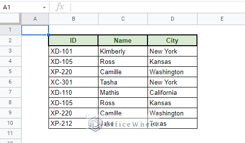
For that we will be extracting the values of the three columns as an array:

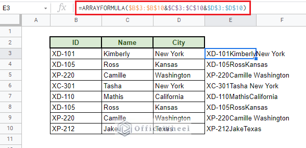
We now have the range for our condition.

Next, we will enclose this range in our COUNTIF function.

For our criterion, we will be using the values of the three columns as a single entity which is free to move down the column. Our criterion formula is: $B3&$C3&$D3

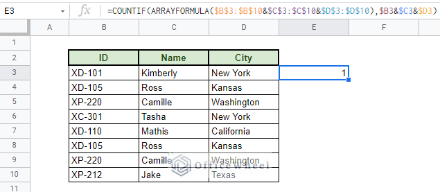
Finally, we add the Boolean condition “>1” to our formula and apply it to the rest of the rows.

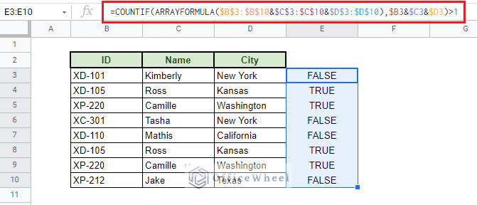
Applying the Conditional Formatting

Now that we have the final version of the formula, we can move forward to applying it to highlight the duplicate instances in our Item list.

Step 1: Select the range and open the Conditional formatting rules menu tray. Format tab> Conditional formatting

Step 2: Apply the custom formula:

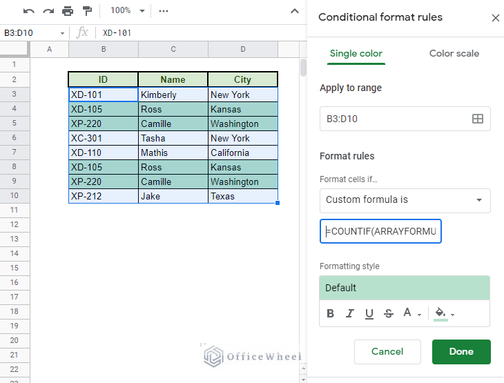
Step 3: Click Done.

We have successfully highlighted all the duplicate rows!

Things to Keep in Mind

1. You can add extra conditions

You can add more conditions to your formula to highlight duplicates. The syntax is something like this:

A new condition can be added after the main count, separated by an asterisk (*). The entire formula must be enclosed within parentheses.

2. Wrong references

You have noticed that we have used a lot of cell references in our formulas. Cell references are an integral part of creating formulas. The three types of cell references we have are:

• Relative References (A1)
• Absolute References ($A$!)
• Mixed References ($A1 or A$1)

To know more about cell references: Lock Cell Reference in Google Sheets

3. Watch out for whitespaces

In Google Sheets, whitespaces are counted as values even if we cannot see them. This may cause some duplicates to be overlooked.

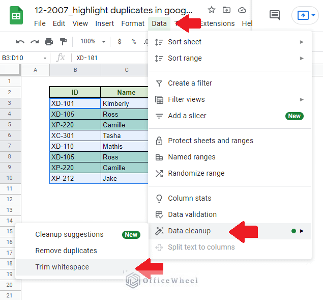
Google Sheets does provide us with an option to Trim Whitespaces.

Data tab > Data Cleanup > Trim Whitespace

Final Words

To round up, to highlight duplicates in Google Sheets can be a bit complicated at first glance, but once you understand how Google Sheets views its data, it becomes fairly easy. Where the actual complication lies is when we are asked to highlight duplicates with unclear and complex values.

We hope that this article has been able to help you understand any queries you might have had regarding highlighting duplicates. If you have any questions, feel free to comment.

Related Articles for Reading

• Conditional Formatting Based on Another Cell in Google Sheets
• Conditional Formatting with Multiple Conditions Using Custom Formulas in Google Sheets
• Count Duplicates In Google Sheets (3 Ways)