Highlight Duplicates in Two Columns in Google Sheets (2 Ways)

While working with a large volume of data in Google Sheets one may encounter duplication of data in their table. They might want to highlight duplicates according to their preference. But highlighting duplicates manually can be very tiring and time-consuming if you have a large volume of data. In this article, we will try to show you how you can highlight duplicates in two columns in Google Sheets very easily.

Table of Contents

A Sample of Practice Spreadsheet

Highlight Duplicates in Two Columns

2 Ways to Highlight Duplicates in Two Columns in Google Sheets

For our approach, Conditional Formatting gives the easiest solution to highlight two columns in Google Sheets.

This feature returns the duplicates between two columns and shows them highlighted. We can access this feature from the format tab:

Format > Conditional formatting

And the Conditional formatting menu looks like this:

We can use conditional formatting in two ways (custom formulas) to achieve our objective.

1. Using MATCH Function Custom Formula in Conditional Formatting

Conditional formatting can be used with the MATCH function to create a custom formula to highlight duplicates in two columns in Google Sheets.

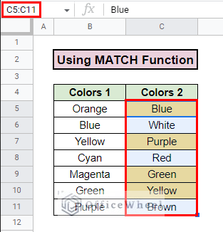
Here we have a dataset with two columns Colors 1 and Colors 2. We want to see if there are any duplicate names from Colors 1 column in the Colors 2 column and highlight the duplicates using Conditional formatting and the MATCH function.

Simply follow these steps:

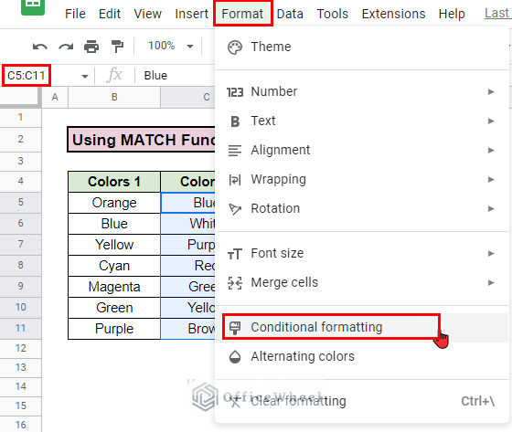
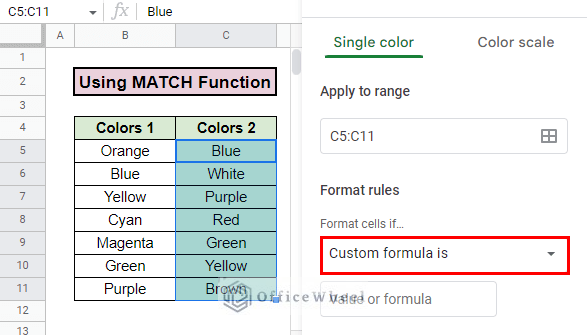
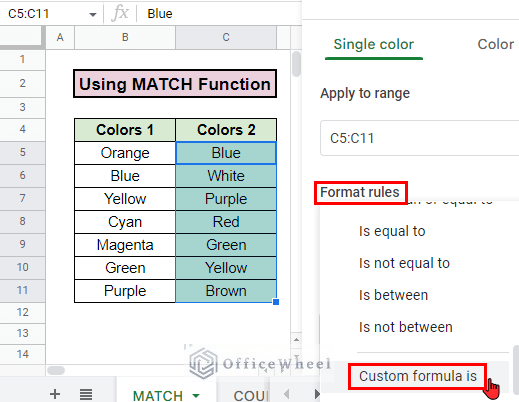
First, select the column where you want to highlight the duplicates and go to Menu bar > Format > Conditional formatting. We select column C5:C11 and go to Format > Conditional formatting.

Then, you should see a sidebar appear from the right named Conditional format rules.

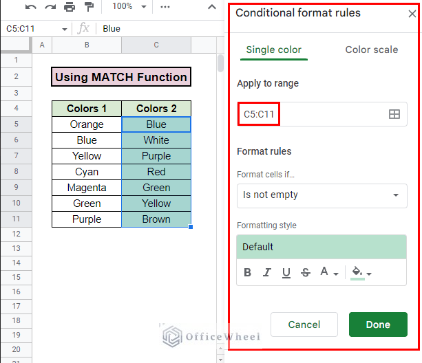
The sidebar specifies where it is applying the Conditional formatting in the Apply to range box. In our example, it says C5:C11.

Next, from the Format rules tab from Format cells if box select Custom Formula is option.

Then, in the Value or formula box type in the MATCH formula based on which the Conditional formatting will highlight the results. We type the following formula:

=MATCH(C5,$B$5:$B$11,0)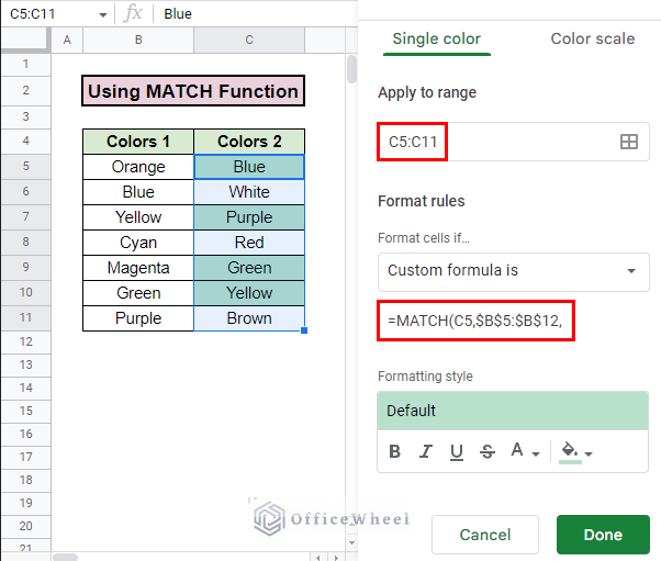

Formula Breakdown:

C5 indicates the cell that the conditional formatting will look for in our main column.
B5:B11 indicates the column in which to look for duplicates. We fixed our column range by the $ sign in front of both the columns and rows name so that it doesn’t change.
0 return the exact matches for our condition. If it doesn’t find a match it won’t highlight anything.

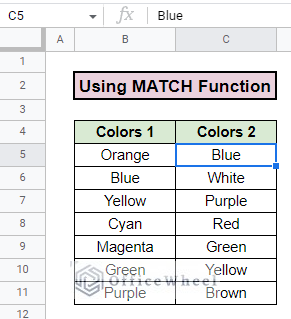
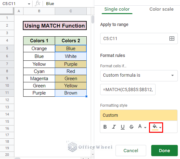
Now, you can change the highlighter color if you want. In this case, we select light yellow 2.

Finally, press Done when you are satisfied with your conditional formatting.

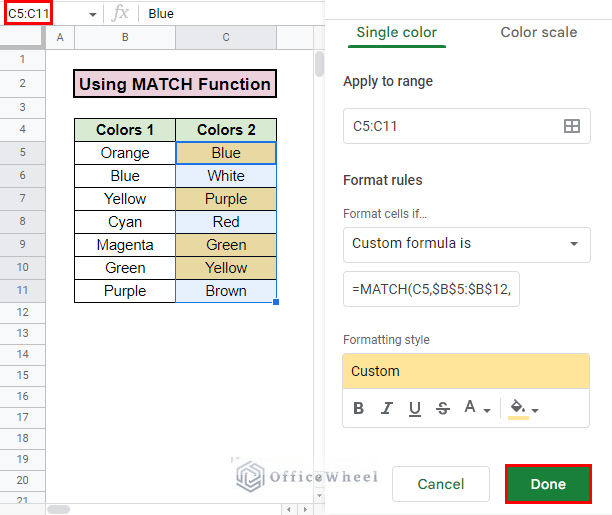
Your duplicates are now highlighted:

Similar Reading

2. Utilizing the COUNTIF Function Custom Formula in Conditional Formatting

Conditional formatting can be applied along with the COUNTIF function to highlight duplicates in two columns in Google Sheets.

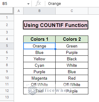
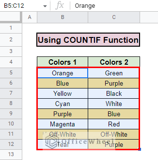
To show this approach, we have a dataset with two columns: Colors 1 and Colors 2. We want to see if there are any duplicate names in the two columns Colors 1 and Colors 2 and highlight the duplicates using Conditional formatting and the COUNTIF function.

Follow these steps carefully:

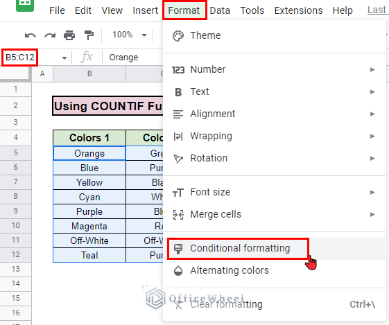
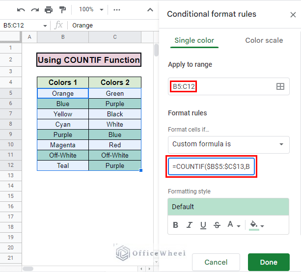
First, select the column range where you want to highlight the duplicates and go to Menu bar > Format > Conditional formatting. We select range B5:C12 and go to Format > Conditional formatting.

Then, you should see a sidebar appear from the right named Conditional format rules.

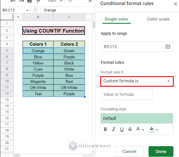
The sidebar specifies where it is applying the Conditional formatting in the Apply to range In our example, it says B5:C12 because we already selected B5:C12.

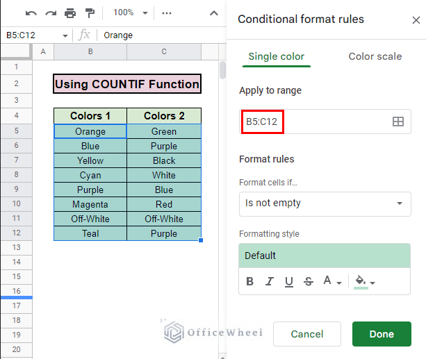
Next, from the Format rules tab from Format cells if box select Custom Formula is option.

Then, in the Value or formula box type in the COUNTIF function formula based on which the Conditional format will highlight the results. We type the following formula:

=COUNTIF($B$5:$C$13,B5)>1

Formula Breakdown:

B5:C13 indicates the range where to look for duplicates in our dataset. We used absolute cell reference for this so that the cell ranges do not change.
B5 denotes the cell reference that the COUNTIF function matches with the table.
As we want any names that match more than once so we type >1 and it will show us the results that are there more than once.

Next, you can change the highlighter color if you want. We select light yellow 2 in this case.
Finally, press Done.

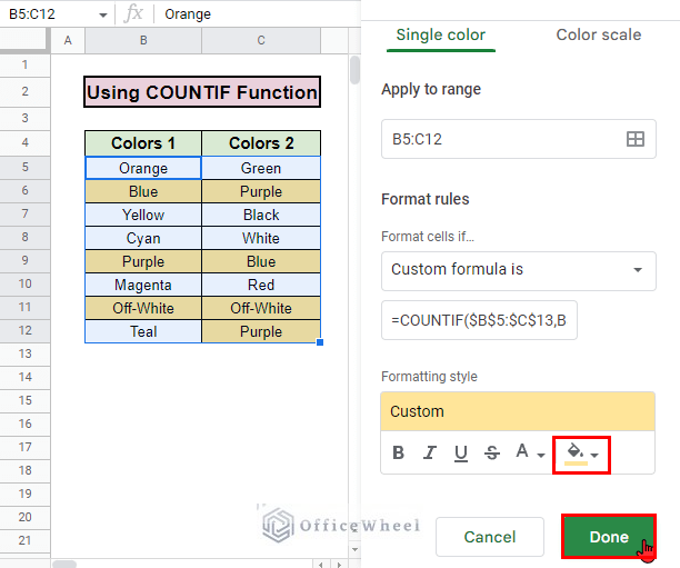
Your duplicates are now highlighted.

Tips and Potential Problems with Solution

The following problems you could face while applying Conditional formatting to highlight duplicates in two columns in Google Sheets:

Extra spaces in the cells may lead to unwanted or non-highlighted cells. For this, you can use the TRIM function to remove extra spaces.
You must use the necessary cell references to make the highlights work properly. Use absolute cell references ($) when possible.
Make sure you do not have any other forms of Conditional formatting applied to the cells.

Conclusion

In this article, we showed you how to highlight duplicates in two columns in Google Sheets. We hope this article was useful to you. Keep on practicing the methods that were shown here to get a grip on the concept.

Also, check out other articles on OfficeWheel to keep on improving your Google Sheets work knowledge.