The VLOOKUP is one of the handiest operations in Google Sheets and Excel. This operation is performed we need to search or extract information from a large dataset. There are several functions like the VLOOKUP, XLOOKUP, or a combination of INDEX and MATCH functions, etc. which can perform the VLOOKUP operation. However, if a dataset contains several matches for any specific value, then the usual VLOOKUP operation will return only the first match. So, is there any way to return the last match? The answer is a resounding Yes and in this article, I’ll discuss 5 simple ways that will help you to VLOOKUP the last match in Google Sheets.
A Sample of Practice Spreadsheet
You can copy our practice spreadsheets by clicking on the following link. The spreadsheet contains an overview of the datasheet and an outline of the described ways to VLOOKUP the last match in Google Sheets.
5 Simple Ways to VLOOKUP Last Match in Google Sheets
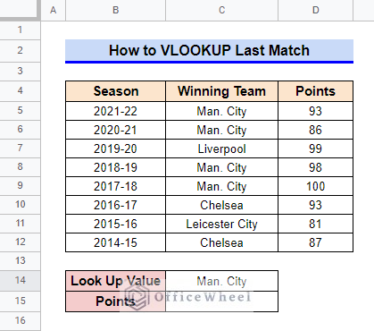
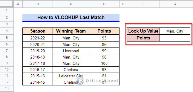
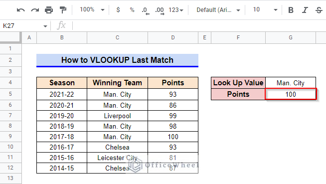
First, let’s get familiar with our dataset. The dataset contains the list of English Premier League winning teams for the last few seasons and their points at the end of that season. We will use a winning team name as a lookup value and return the points for the last match. Now keep reading the following methods.
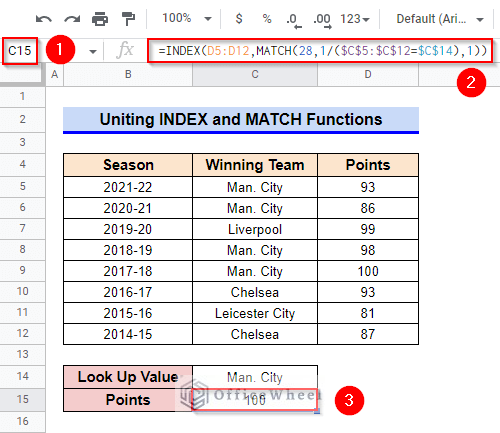
1. Uniting INDEX and MATCH Functions
A simple way to VLOOKUP the last match in Google Sheets is to unite the INDEX and MATCH functions. Although, we will use the arguments of the MATCH function a bit differently to extract the last match.
Steps:
- First, select Cell C15.
- Afterward, type in the following formula:
=INDEX(D5:D12,MATCH(28,1/($C$5:$C$12=$C$14),1))- Finally, press Enter key to get the required result.
Formula Breakdown
- MATCH(28,1/($C$5:$C$12=$C$14),1)
First, the MATCH function searches for a random value 28 in the search range. But a match will not be found since the provided range 1/($C$5:$C$12=$C$14) will return either 1 or #DIV/0! error. Therefore, the MATCH function will return the relative position of the last non-error cell and this will help the INDEX function to return the last match.
- INDEX(D5:D12,MATCH(28,1/($C$5:$C$12=$C$14),1))
Then, from range D5:D12, the INDEX function returns the cell’s content with an index returned by the MATCH function.
Read More: How to Use the VLOOKUP Function in Google Sheets
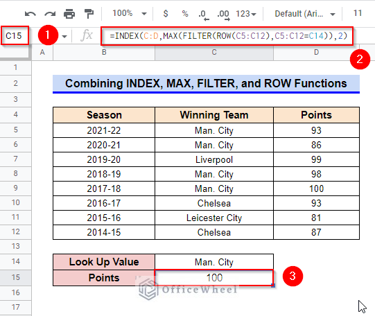
2. Combining INDEX, MAX, FILTER, and ROW Functions
Another way to return the last match from a dataset is to combine the INDEX, MAX, FILTER, and ROW functions.
Steps:
- Select Cell C15
- After that, type in the following formula:
=INDEX(C:D,MAX(FILTER(ROW(C5:C12),C5:C12=C14)),2)- Then, press Enter key to get the required result.
Formula Breakdown
- ROW(C5:C12)
First, the ROW function returns the row number for each cell within the range C5:C12.
- FILTER(ROW(C5:C12),C5:C12=C14)
Afterward, the FILTER function returns the index of the rows where the condition specified by C5:C12 = C14 is true.
- MAX(FILTER(ROW(C5:C12),C5:C12=C14))
Then, the MAX function returns the maximum row number (which is in the last match) in the dataset returned by the FILTER function.
- INDEX(C:D,MAX(FILTER(ROW(C5:C12),C5:C12=C14)),2)
Finally, the INDEX function returns the cell’s content with an index returned by the MAX function.
Read More: Combine VLOOKUP and HLOOKUP Functions in Google Sheets
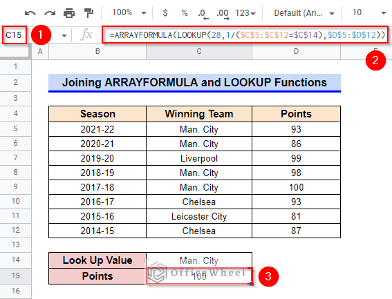
3. Joining ARRAYFORMULA and LOOKUP Functions
The LOOKUP function can also find the last occurrence of a string in a dataset. Since the LOOKUP function is a non-array function, we have to join the ARRAYFORMULA function with it.
Steps:
- To start with, select Cell C15.
- Afterward, type in the following formula:
=ARRAYFORMULA(LOOKUP(28,1/($C$5:$C$12=$C$14),$D$5:$D$12))- Finally, press Enter key to get the required result.
Formula Breakdown
- LOOKUP(28,1/($C$5:$C$12=$C$14),$D$5:$D$12)
Here, the LOOKUP function searches for a random value of 28 in the search range. But a match will not be available since the given range 1/($C$5:$C$12=$C$14) will return either 1 or #DIV/0! error. Therefore, the LOOKUP function will return the relative position of the last non-error cell and this will help the INDEX function to return the last match.
- ARRAYFORMULA(LOOKUP(28,1/($C$5:$C$12=$C$14),$D$5:$D$12))
The LOOKUP function is a non-array function. Therefore, the ARRAYFORMULA function helps the LOOKUP function deal with arrays.
Read More: How to Use ARRAYFORMULA with VLOOKUP in Google Sheets
Similar Readings
- How to Use ARRAYFORMULA in Google Sheets (6 Examples)
- VLOOKUP All Matches in Google Sheets (2 Approaches)
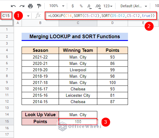
4. Merging LOOKUP and SORT Functions
Merging a LOOKUP function and two SORT functions can also help you to VLOOKUP the last match in Google Sheets.
Steps:
- First, select Cell C15.
- After that, type in the following formula:
=LOOKUP(C14,SORT(C5:C12),SORT(D5:D12,C5:C12,true))- In the end, press Enter key to get the required result.
Formula Breakdown
- SORT(C5:C12)
To start with, the first SORT function sorts the search range C5:C12.
- SORT(D5:D12,C5:C12,true)
Then, the second SORT function sorts the result range D5:D12 considering C5:C12 already sorted.
- LOOKUP(C14,SORT(C5:C12),SORT(D5:D12,C5:C12,true))
Finally, the LOOKUP function returns the last match cell’s content for Cell C14.
Read More: How to Merge Columns in Google Sheets
5. Using Apps Script
You can also write a simple script to VLOOKUP the last match in Google Sheets. To execute our script properly, we have modified our dataset.
Steps:
- First, go to the Extensions ribbon and select Apps Script from the options.
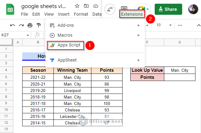
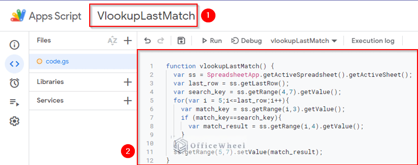
- A new window like the following will open in your browser.
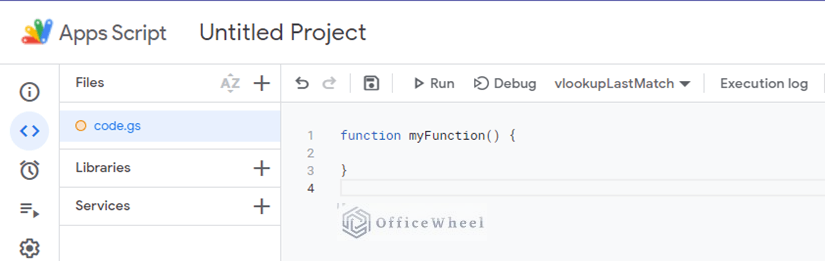
- Rename the project and enter the following script:
function vlookupLastMatch() {
  var ss = SpreadsheetApp.getActiveSpreadsheet().getActiveSheet();
  var last_row = ss.getLastRow();
  var search_key = ss.getRange(4,7).getValue();
  for(var i = 5;i<=last_row;i++){
    var match_key = ss.getRange(i,3).getValue();
    if (match_key==search_key){
      var match_result = ss.getRange(i,4).getValue();
    }
  }
  ss.getRange(5,7).setValue(match_result);
}
- After that, Save and Run the project. Provide the required permissions.
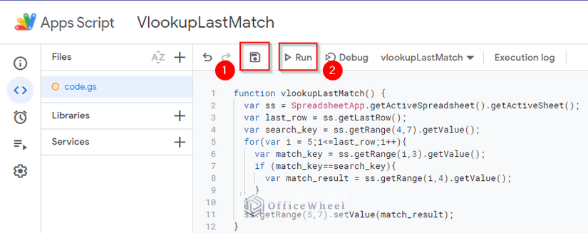
- The last match will be updated in the required cell.
Read More: How to VLOOKUP with Multiple Criteria in Google Sheets
Things to Be Considered
- Remember to fix the required cells while using method 1 and method 3.
- The LOOKUP function is not an array function. Therefore, join it with the ARRAYFORMULA function if you need to deal with an array while using the LOOKUP
- Provide required permissions to run the script while using Apps Script.
- Turn on the Iterative Calculation option from the File ribbon if required.
Conclusion
This concludes our article to learn how to VLOOKUP the last match in Google Sheets. I hope the article was sufficient for your requirements. Feel free to leave your thoughts on the article in the comment box. Visit our website OfficeWheel.com for more useful videos.
Related Articles
- VLOOKUP Between Two Google Sheets (2 Ideal Examples)
- How to Use VLOOKUP with Named Range in Google Sheets
- Alternative to Use VLOOKUP Function in Google Sheets
- How to Concatenate with VLOOKUP in Google Sheets
- VLOOKUP Multiple Columns in Google Sheets (3 Ways)
- How to Sum Using ARRAYFORMULA in Google Sheets