Create Hyperlink to VLOOKUP Cell in Multiple Rows in Google Sheets

Suppose you may need to work between different datasets at the same time in Google Sheets. Switching the dataset manually every time is a time-consuming job. This might also cause difficulties for people who are new and learning something. In that case, you can create a hyperlink to the VLOOKUP output to directly jump into the sheet which needed that time. In this article, we will learn how to create a hyperlink to the output cell obtained from applying VLOOKUP on multiple rows in Google Sheets.

A Sample of Practice Spreadsheet

You may copy the spreadsheet below and practice by yourself.

Introduction to HYPERLINK Function in Google Sheets

The HYPERLINK function is used to create a hyperlink that can jump from one place to another in a sheet or show the source sheet.

Syntax

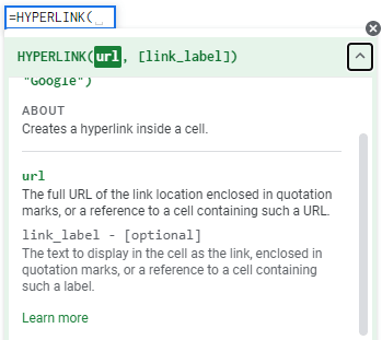
Arguments

• url: Here, the full URL of a cell is required which will be enclosed in double quotes as a reference.
• [link_label]: It shows the display as a link.

Return Value

• Returns the value as a hyperlink.

3 Examples of Creating Hyperlink to VLOOKUP Cell in Multiple Rows in Google Sheets

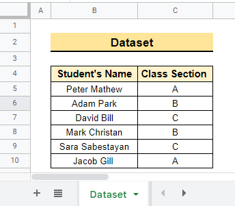
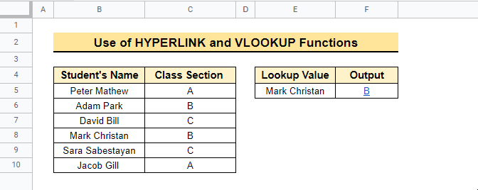
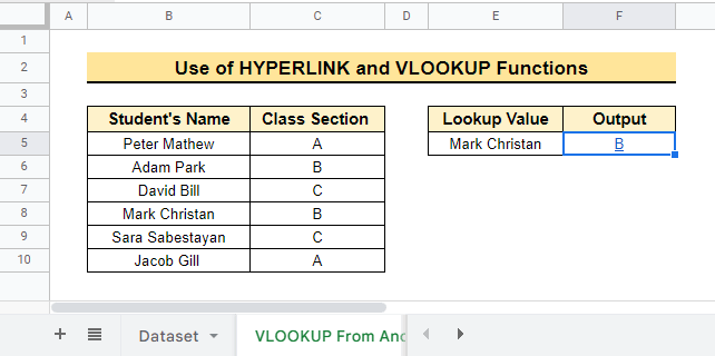
The dataset below has multiple rows containing Student’s Name and Class Section.  We will use this dataset to create a hyperlink to the output cell obtained from applying VLOOKUP on multiple rows in Google Sheets.

Follow the examples below to understand the methods properly.

1. Creating Hyperlink to VLOOKUP Cell in Same Sheet

Here, we will create a hyperlink to the VLOOKUP cell within multiple rows in the same sheet. The steps are mentioned below.

📌 Steps:

• First, select cell F5 and enter the VLOOKUP function using cell E5 as the lookup value.

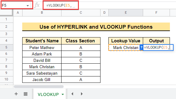
• Then, select range B5:C10 in the same sheet as the lookup range.

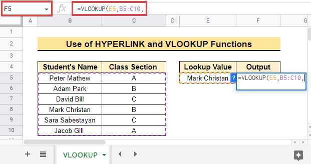
• After that, type 2 for the index and complete the VLOOKUP formula by typing 0 to get the exact match.

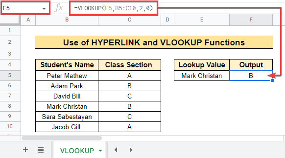
• Now, use the earlier formula as the reference argument of the CELL function to get the cell address of the output as below.

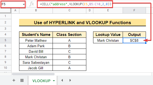
• Here, $C$8 is the cell address of the VLOOKUP But to execute the formula, you need to convert the cell address into cell reference C8 using the SUBSTITUTE function to remove the $ sign as below.

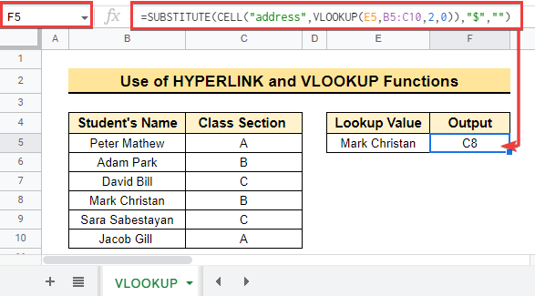
After that, you need to create a dynamic hyperlink to the output cell. To create the hyperlink follow the steps below.

• First, select a blank cell in the existing sheet. For example, right-click on cell J7 in the sheet containing the VLOOKUP
• Then select View more cell actions >> get link to the cell and the URL of the cell will be copied to the clipboard.

• Now paste the link and it will show the cell number at the end of the link as ("https://docs.google.com/spreadsheets/d/1T1AexOGSR7WpBX7JO8Rvahs6F78UBTojFm8vcrIiUxg/edit#gid=232756586&range=J7"). Then remove the cell reference J7 from the end of the link. Next, type a & symbol after the link and then paste the earlier formula as "https://docs.google.com/spreadsheets/d/1T1AexOGSR7WpBX7JO8Rvahs6F78UBTojFm8vcrIiUxg/edit#gid=232756586&range="&SUBSTITUTE(Cell("address",VLOOKUP(E5,B5:C10,2,0)),"$","").
• Next, insert the HYPERLINK function in cell F5 and use the modified link above as the URL argument of the function.

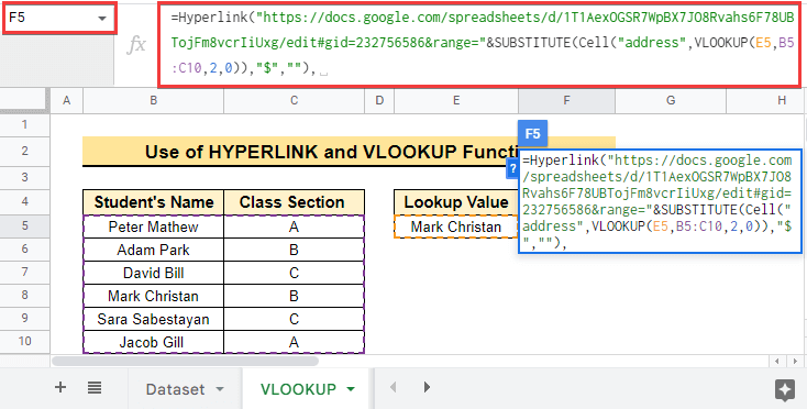
• After that, use the VLOOKUP(E5,B5:C10,2,0) formula as the link_label argument of the HYPERLINK function. Finally, enter the formula to see the hyperlink as follows.

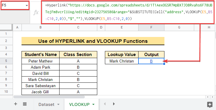
• Now click on the hyperlink to jump to the actual cell containing the output value within the dataset.

Read More: How to VLOOKUP Multiple Columns in Google Sheets (3 Ways)

Similar Readings

• How to Concatenate with VLOOKUP in Google Sheets
• Do Reverse VLOOKUP in Google Sheets (4 Useful Ways)
• How to Use VLOOKUP with IF Statement in Google Sheets
• Check If Value Exists in Range in Google Sheets (4 Ways)
• How to Use VLOOKUP with Drop Down List in Google Sheets

2. Building Hyperlink to VLOOKUP Cell in Another Sheet

Here, we will build a hyperlink to the VLOOKUP cell within multiple rows in another sheet in the same spreadsheet. Follow the steps below to do that.

📌 Steps:

• First, enter the VLOOKUP function using cell E5 as the lookup value and Dataset!B5:C10 as the lookup range.
• Then, type 2  for the index and complete the VLOOKUP formula by typing 0 to get the exact match.

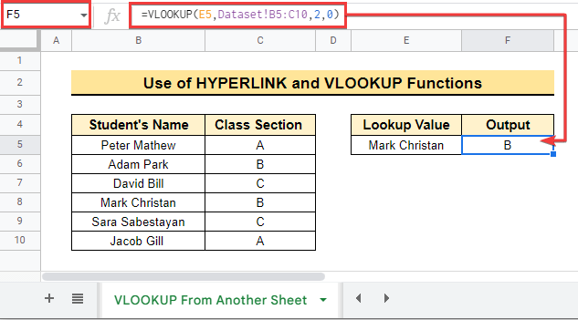
• Now, use the earlier formula as the reference argument of the CELL function to get the cell address of the output as below.

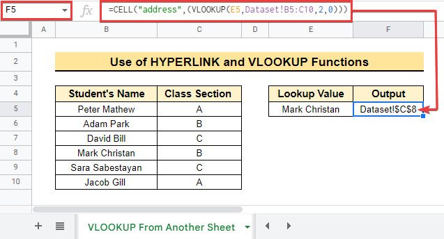
• Here, Dataset!$C$8 is the cell address for the output value. But to execute the formula, convert the cell address into cell reference C8 using the nested SUBSTITUTE function (nested function is used when you need to add more logic using the same function) and remove the sign “$ as below.

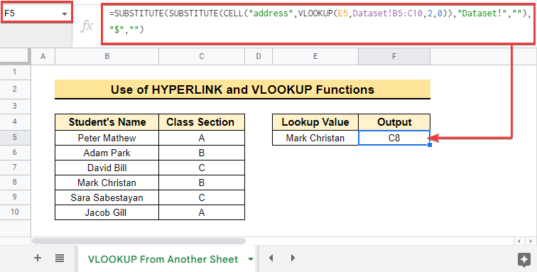
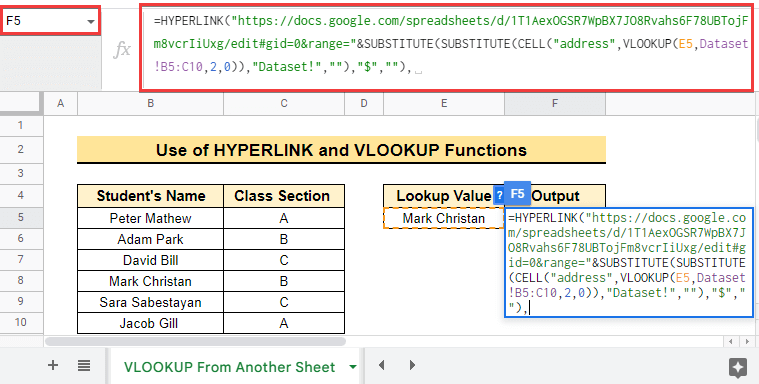
• Now right-click on a cell and select View more cell actions >> get link to the cell to to create a Dynamic hyperlink following the steps shown before.
• After that, modify the link as "https://docs.google.com/spreadsheets/d/1T1AexOGSR7WpBX7JO8Rvahs6F78UBTojFm8vcrIiUxg/edit#gid=0&range="&SUBSTITUTE(SUBSTITUTE(CELL("address",VLOOKUP(E5,Dataset!B5:C10,2,0)),"Dataset!",""),"$","") and use it as the URL argument for the HYPERLINK function.

• Then, use the VLOOKUP(E5,Dataset!B5:C10,2,0) formula as the link_label argument of the HYPERLINK Finally, enter the formula to see the hyperlink as follows.

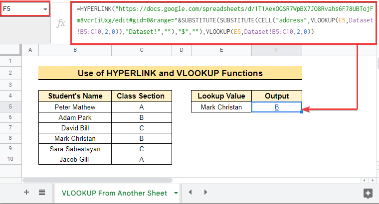
• Now click on the hyperlink to jump to the actual cell containing the output value within the dataset.

Read More: How to VLOOKUP from Another Sheet in Google Sheets (2 Ways)

3. Combining HYPERLINK and VLOOKUP Functions

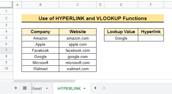
The dataset below contains Company names and a link-like text of the corresponding Website. We will get the hyperlink of this website using the HYPERLINK and VLOOKUP functions. Lets Start.

📌 Steps:

• Select cell F5 and enter the VLOOKUP function using cell E5 as the lookup value and cell range B5:C10 as the lookup range.
• Then, type 2  for the index and complete the VLOOKUP formula by typing 0 to get the exact match.

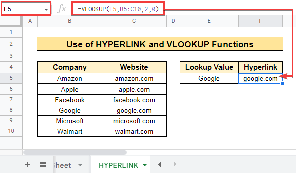
• After that, insert the HYPERLINK function before the earlier formula to convert the output to a clickable hyperlink and the output will be as below.

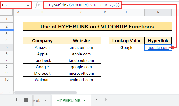
Read More: Combine VLOOKUP and HLOOKUP Functions in Google Sheets

Things to Remember

• Always remember to enclose the hyperlink within double quotes.
• Write down the sheet name manually within double quotes if you VLOOKUP from another sheet.

Conclusion

In this article, we explained the anatomy of the VLOOKUP function. We also explained how to create a hyperlink to the output cell obtained from applying VLOOKUP on multiple rows in Google Sheets. Hopefully, the examples will help you to apply this method to your own dataset. Please let us know in the comment section if you have any further queries or suggestions. You may also visit our OfficeWheel blog to explore more Google Sheets-related articles.

Related Articles

• How to Use Nested VLOOKUP in Google Sheets
• [Fixed!] Google Sheets If VLOOKUP Not Found (3 Suitable Solutions)
• How to VLOOKUP Between Two Google Sheets (2 Ideal Examples)
• Check If Value Exists in Range in Google Sheets (4 Ways)
• How to Use IFERROR with VLOOKUP Function in Google Sheets
• Use VLOOKUP to Import from Another Workbook in Google Sheets
• How to VLOOKUP Last Match in Google Sheets (5 Simple Ways)
• Use VLOOKUP for Conditional Formatting in Google Sheets