How to Use IFERROR with VLOOKUP Function in Google Sheets

An essential component of data processing is error handling. Errors are typically often possible when doing data operations. While using VLOOKUP, we occasionally discover mistakes. Fortunately, Google Sheets can detect these mistakes and tell you with an error code. One of the well-designed and user-friendly functions in Google Sheets to fix and conceal errors made while doing a VLOOKUP is the IFERROR function.

A Sample of Practice Spreadsheet

You can copy our spreadsheet that we’ve used to prepare this article.

What Is IFERROR Function in Google Sheets?

In Google Sheets, the IFERROR function can display any error, incorrect or missing value in VLOOKUP in a logical fashion. The IFERROR Function can offer a viable solution if everything appears to be in order but the formula still fails to return the desired value.

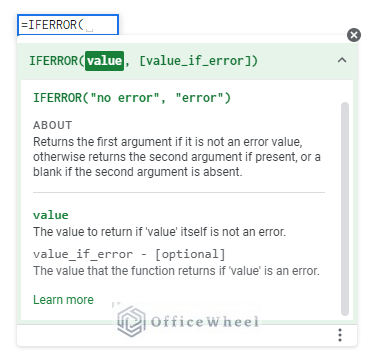
When there is no error value, the IFERROR function in Google Sheets typically returns the first parameter; otherwise, it returns the second argument or a blank if the second argument is missing. To comprehend how to use the IFERROR function with VLOOKUP, refer to the section after this one.

3 Practical Examples to Use IFERROR with VLOOKUP Function in Google Sheets

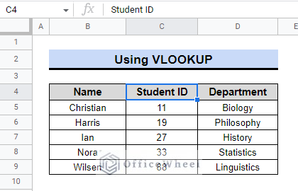
We’ll use a basic dataset to show how to use the IFERROR function in the context of VLOOKUP. Let’s say we have information about a few university students. We will conduct a search using the VLOOKUP function to locate some specific data.

Steps:

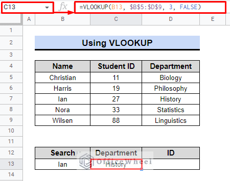
• First, we will choose cell C13.
• Second, we’ll apply the formula shown below:

• Finally, press ENTER to finish.

In the end, we will discover that the VLOOKUP formula will use the search column to display the relevant information whenever we type a name. However, occasionally it will display errors. Let’s look at a few examples below.

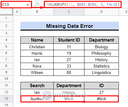
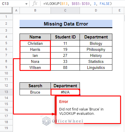
Example 1: Missing Data Error

Assume we’re looking for information about a student named Aurthur. The VLOOKUP function, however, displays a “#N/A” error. This implies that no information on the name is available.

We will now apply the following formula to transform the error message into a more systematic and logical approach.

Steps:

• We shall first choose cell C13.
• The prior formula will remain in place. However, we will remedy the scenario by implementing the IFERROR function around the existing VLOOKUP formula.
• We’ll use the following formula:

• Lastly, click ENTER.

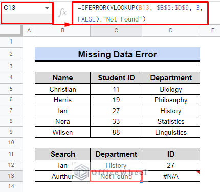
The error value is no longer present, as shown in the image. Instead, the designated cells show the phrase “Not found.” We may therefore use IFERROR with VLOOKUP for a more structured process if there is no data.

Read More: [Fixed!] IFERROR Function Is Not Working in Google Sheets

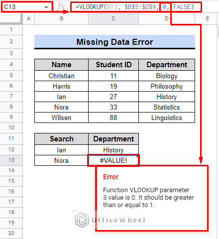
Example 2: Incorrect Column Reference

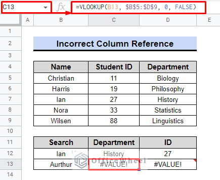
When entering data into a formula, we tend to make mistakes occasionally. Using the wrong column references when using VLOOKUP is one of the common blunders people make.

We encountered errors like #VALUE! while looking for information about Aurthur. It signifies that the value in the formula is inaccurate and misleading. In this case, a column reference that should be greater than 1 has been inserted as 0.

To reconstruct the error methodically and logically, we will now use the formula shown below.

Steps:

• At first, we will select cell C13.
• We’ll use the following formula in order to resolve the error.

• To finish, click ENTER.

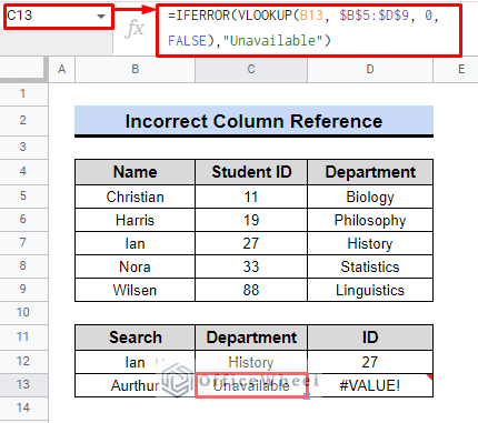
As seen in the image, the error warning has simply disappeared. Instead, “Unavailable” is displayed in the designated cell. Similarly, we can handle the error message in cell D13. The steps are as follows:

• Select cell D13 once more.
• We’ll apply the following formula.

• Finally, press the ENTER key to finish.

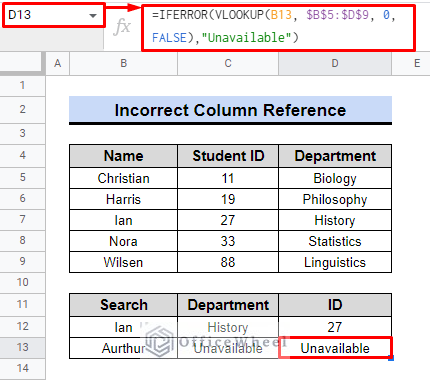
Now, Aurthur-related information is handled as Unavailable, as you can see in the image above. This seems more presentable than the previous predicament.

Example 3: Error in the Formula

Consider the possibility that we are unaware of a data or formula parse error. Therefore, it displays a “#ERROR” message while running VLOOKUP.

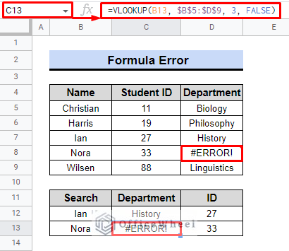
We will go through the same procedure again to temporarily fix the problem.

Steps:

• We’re going to choose cell C13 once more.
• Following that, we’ll utilize the following formula without altering the VLOOKUP formula.

• Press ENTER to finish after that.

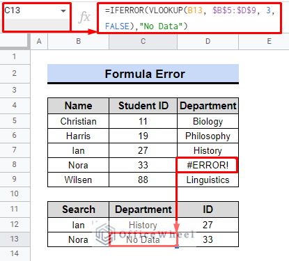
We can see from the image that the error result is no longer present. However, if we look at the source data range, we can quickly identify the issue. Thus, by using the IFERROR function, we can address issues that occurred when executing VLOOKUP.

Most Common VLOOKUP Errors in Google Sheets

VLOOKUP is one of the most helpful yet challenging features in Google Sheets. It aids in the search for similar data across numerous sheets. However, your formula could occasionally produce errors. Here are some lists of common errors in VLOOKUP.

I. #N/A Error for Incorrect Data

This error most frequently occurs in Google Sheets VLOOKUP and indicates that the value is unavailable, misspelled, or mismatched.

II. #VALUE! Error for Incorrect Column Number

In Google Sheets VLOOKUP, the third argument can occasionally be specified incorrectly. It should fall between 1 and the total number of columns included in the search range. VLOOKUP in Google Sheets will return the #VALUE! error if the number is incorrect.

III. #REF! Error in Case of Invalid Reference to Another Table

If you encounter the #REF! error, you’ll realize that something is wrong. It denotes that the formula cannot locate the range you entered because it is invalid.

IV. #ERROR If Mistakes Occur in Formula

It is known as a formula phase error message and is exclusive to Google Sheets. It indicates that Google Sheets is unable to understand the formula you have entered because it is unable to parse the formula to execute it.

Things to Remember

The function has the drawback of treating all error messages the same and not differentiating between them. As a result, other users may find it difficult to diagnose the issues because they won’t be aware of the nature of the problem. Because of this, it often creates confusion like the function IFERROR is not working properly in google sheets.

The IFERROR function serves as a general solution for all VLOOKUP errors and mistakes. It should handle any errors or exceptions in Google Sheets.

Final Words

The IFERROR function acts as a general remedy for all errors. You could run into the two issues listed above while using VLOOKUP in Google Sheets, IFERROR is quite effective in these situations and handles these errors similarly. Please leave a comment if you have any questions. For more interesting and important articles, please visit OfficeWheel.

Related Article

• [Fixed!] IFERROR Function Is Not Working in Google Sheets