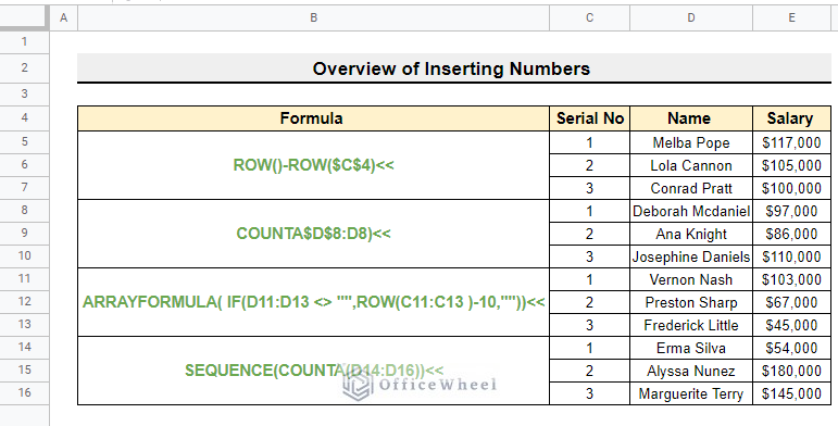
Inserting numbers or serial numbers in Google Sheets is very simple and easy. But there are various ways to do it. And some methods are useful depending on the nature of the data. This article gives you a comprehensive idea of how to insert numbers in Google Sheets in usual cases as well as in some special cases depending on the data you are working on.
A Sample of Practice Spreadsheet
You can download the spreadsheets from the link below. The spreadsheets contain a dataset we use here. After downloading you can practice on your own as we demonstrate here.
7 Easy Ways to Insert Serial Numbers in Google Sheets
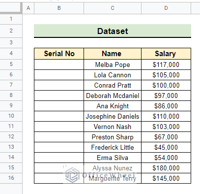
There are various ways of inserting numbers in Google Sheets. We are going to discuss seven different methods of how to insert numbers using the following dataset.
1. Double-Clicking Fill Handle Icon
The easiest and quickest way to insert serial numbers in Google Sheets is by double-clicking on the fill handle tool. But we need to insert the first two numbers of the serial manually.
📌 Steps:
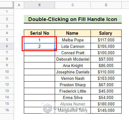
- First of all, we insert the first two serials manually in the first two cells like in the image below.
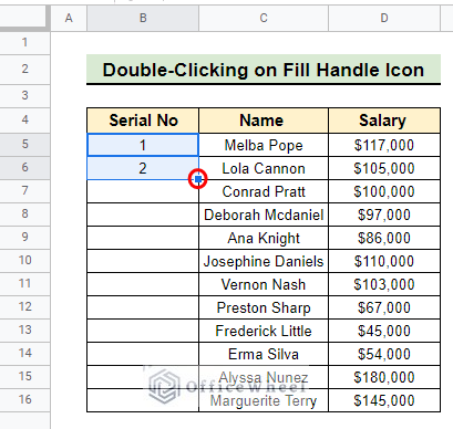
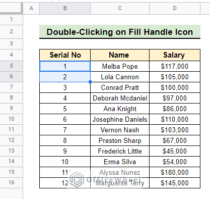
- Then we select the first two serial numbers that we already inserted and double-click on the fill handle icon as indicated.
- As a result, all the rows of the Serial No column are filled with their corresponding serial number.
Read More: Insert Rows Between Other Rows in Google Sheets (4 Easy Ways)
2. Dragging Down the Fill Handle
In this method, we are going to employ the previous method but in a different way. Instead of double-clicking, we drag down the fill handle to insert serial numbers in Google Sheets.
📌 Steps:
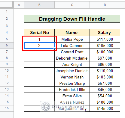
- At the very beginning, we insert the first two serials manually in the first two cells like in the image below.
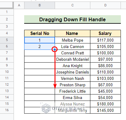
- Next, we select the first two serial numbers that we already inserted and drag down the fill handle as follows.
- Consequently, we get the Serial No for the rows other than the first two rows.
Read More: How to Have More than 26 Columns in Google Sheets
3. Adding One to the Previous Number
The next way to insert serial numbers in Google Sheets involves the use of the SUM function.
📌 Steps:
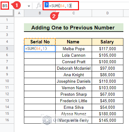
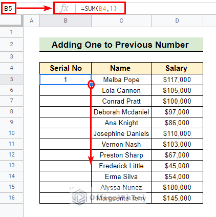
- Firstly, we select cell B5.
- After that, we write down the following formula in the formula bar.
=SUM(B4,1)- Hence, we get the first serial number in the selected cell.
- Next, we use the fill handle tool to get the serial number of the subsequent rows.
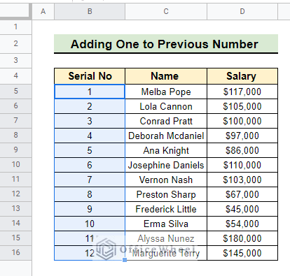
- Once we complete the fill handle operation, we get the following result.
Read More: How to Insert Formula in Google Sheets for Entire Column
Similar Readings
- How to Insert Multiple Columns in Google Sheets (2 Quick Ways)
- Insert an Exponent in Google Sheets (3 Easy Ways)
- How to Insert a Legend in Google Sheets (With Easy Steps)
- Insert Signature in Google Sheets (3 Easy Ways)
- How to Insert a Calendar in Google Sheets (2 Effective Ways)
4. Using the ROW Function
The ROW function is another useful technique for inserting serial numbers in Google Sheets. In this method, we are going to demonstrate how to insert serial numbers with a few easy steps described below.
📌 Steps:
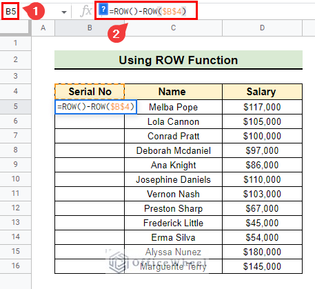
- At first, we select cell B5.
- Afterward, we insert the formula below in the formula bar.
=ROW()-ROW($B$4)
- Here we are subtracting the row number of cell B4 from the first row of our data because our first data is in the 5th row of the spreadsheet.
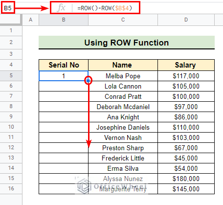
- Thus we get the serial number in the selected cell.
- Then we drag down the fill handle to fill the subsequent rows with the corresponding serial number.
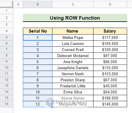
- Finally, we get the desired serial number inserted as follows.
Read More: How to Insert Multiple Rows in Google Sheets (4 Ways)
5. Applying COUNTA Function
We can apply the COUNTA function as well to insert serial numbers in Google Sheets. For this, we need to follow the steps described below.
📌 Steps:
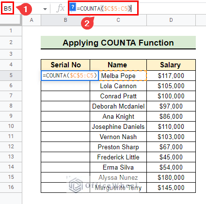
- Initially, we select cell B5 as earlier.
- Next, we insert the formula below in the formula bar.
=COUNTA($C$5:C5)- As a result, we get the first serial in the selected cell.
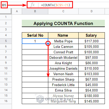
- Afterward, we drag down the fill handle tool to get all the serial numbers.
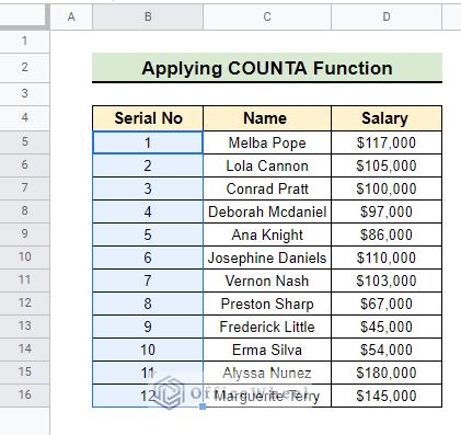
- After completing the fill handle task we get the following result.
6. Utilizing ARRAYFORMULA Function
The next but not the last way of inserting numbers in Google Sheets involves the utilization of the ARRAYFORMULA function. We can get the serial number for the whole dataset just by writing the formula in the formula bar.
📌 Steps:
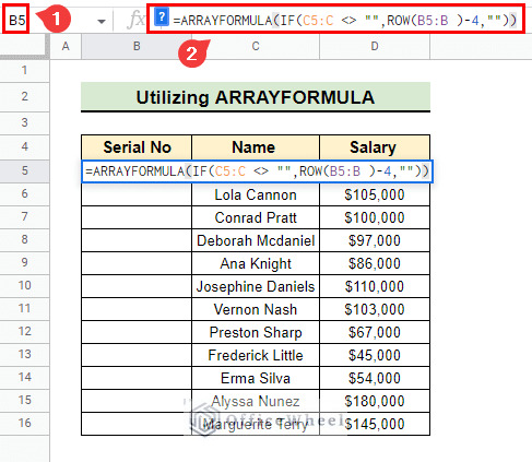
- First of all, we select cell B5.
- Next, we write down the following formula in the formula bar.
=ARRAYFORMULA(IF(C5:C <> "",ROW(B5:B )-4,""))Formula Breakdown
- ROW(B5:B )-4
The ROW function counts the row number for each of column B from cell B5.
Result: 1
- IF(C5:C <> “”,ROW(B5:B )-4,””)
The IF function returns blank if the corresponding cell of Column C is blank.
Result: 1
- ARRAYFORMULA(IF(C5:C <> “”,ROW(B5:B )-4,””))
Finally, the ARRAYFORMULA dynamically fills all the rows with the given formula written inside of it.
Result: 1
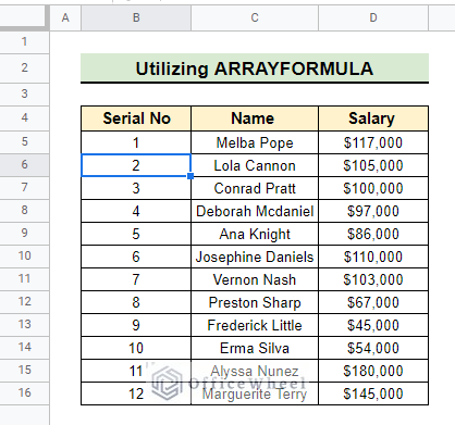
- Finally, we press Enter and get the following result.
Read More: How to Insert Blank Column Using QUERY in Google Sheets
Similar Readings
- How to Insert Gridlines in Google Sheets (4 Suitable Methods)
- Make a Tournament Bracket in Google Sheets (Easy Steps)
- How to Insert PDF in Google Sheets (2 Suitable Methods)
- Insert a Header in Google Sheets (2 Simple Scenarios)
- Insert Page Break in Google Sheets (An Easy Guide)
7. Implementing SEQUENCE Function
The last method we are going to discuss to insert numbers in Google Sheets is the implementation of the SEQUENCE function.
📌 Steps:
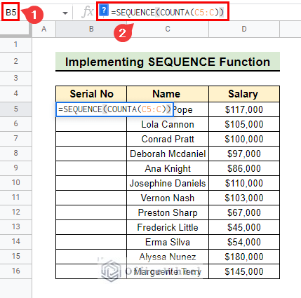
- Initially, we select cell B5 as earlier.
- Next, we insert the formula below in the formula bar.
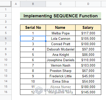
=SEQUENCE(COUNTA(C5:C))- Lastly, pressing the Enter key gives us the following result.
How to Insert Numbers with Blank Rows in Google Sheets
Now, let’s say there is no data for some rows in the middle of our dataset and we still want to insert serial numbers using the COUNTA function. We can easily do that. However, we need a couple of helper functions along with the COUNTA function.
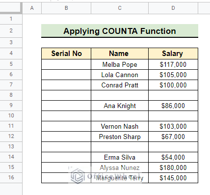
Say, we have some blank rows in our dataset that were previously filled. Now we want to insert serial numbers in the dataset below. Follow the steps below to do this.
📌 Steps:
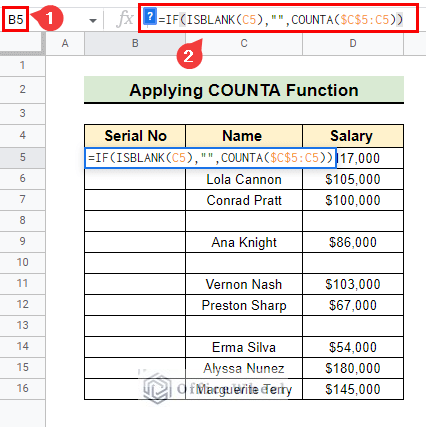
- Here we select cell B5 as usual.
- Then we insert the formula below in the formula bar.
=IF(ISBLANK(C5),"",COUNTA($C$5:C5))Formula Breakdown
- COUNTA($C$5:C5)
The COUNTA function counts the number of cells within the range $C$5:C5.
Result: 1
- ISBLANK(C5)
The ISBLANK function whether the cell C5 within its argument is blank or not.
Result: FALSE
- IF(ISBLANK(C5),””,COUNTA($C$5:C5))
The IF function returns the value of COUNTA($C$5:C5) if the given condition is false.
Result: 1
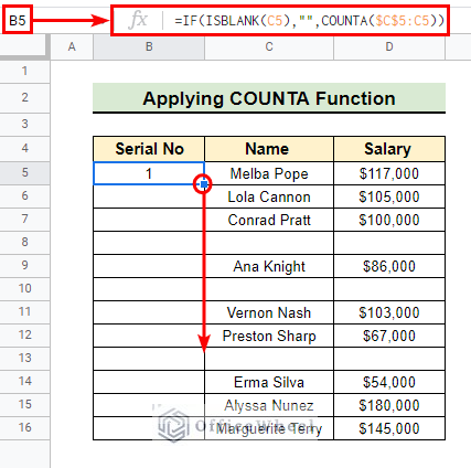
- Consequently, we get the first serial in the selected cell.
- Later we perform the fill handle operation as indicated in the image below.
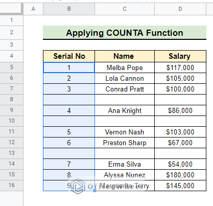
- Thus, we get the serial number in the desired rows. One important thing to notice here is that the formula avoids inserting serial numbers in the blank rows as we already mentioned.
Read More: How to Paste and Insert Rows in Google Sheets (3 Easy Ways)
Things to Remember
Always remember you can’t perfectly insert serial numbers using the ARRAYFORMULA describe here if there are any blank rows.
Conclusion
In conclusion, inserting numbers in Google Sheets is a fairly simple task. I believe from now on you can adopt the best-suited method. Further, If you have any questions regarding this article feel free to comment below and I will try to reach out to you soon. Visit our website OfficeWheel for the most useful articles.
Related Articles
- How to Insert Superscript in Google Sheets (2 Simple Ways)
- Insert Button in Google Sheets (5 Quick Steps)
- How to Add Parentheses in Google Sheets (5 Ideal Scenarios)
- Insert Error Bars in Google Sheets (3 Practical Examples)
- How to Insert Yes or No Box in Google Sheets (2 Easy Ways)
- Insert a Drop-Down List in Google Sheets (2 Easy Ways)
- How to Insert Equation in Google Sheets (4 Tricky Ways)

