How to Insert a Legend in Google Sheets (With Easy Steps)

Users of Google Sheets have access to a wide range of chart types to assist them to visualize their data. However, simply displaying a chart with a lot of colored columns or lines is insufficient. Your chart should be able to make sense to someone who is just looking at it. To explain to the reader what each of these lines, shapes, or colors represents, your chart should also include a legend. The option to put legends and labels in a chart is available in Google Sheets. So, in this article, we’ll see the step-by-step process of how to insert a legend in Google Sheets with clear images and steps. We’ll also see how to customize a legend in Google Sheets. At last, you’ll get an output like the following picture.

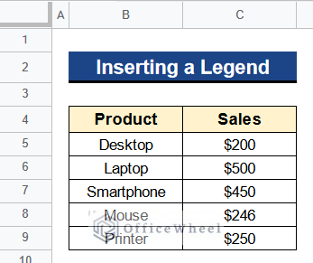
A Sample of Practice Spreadsheet

You can download Google Sheets from here and practice very quickly.

Step-by-Step Process to Insert a Legend in Google Sheets

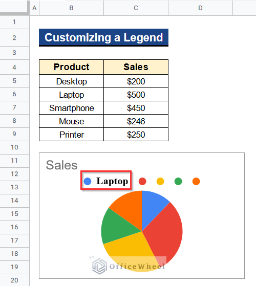
Let’s get introduced to our dataset first. Here we have some products in Column B and their sales prices in Column C. We want to make a chart from this data table and then insert a legend there. Now, I’ll show you the step-by-step process of how to insert a legend in Google Sheets by using this dataset.

Step 1. Create a Chart

First of all, we have to create a chart from our dataset. Then we’ll include a legend in our chart. There are different types of charts available in Google Sheets like Pie Charts, Column Charts, Bar Charts, Line Charts, etc. different charts are used for different purposes. You can include legends in all types of charts. Among these charts, we’ll make a Pie Chart from our dataset. The process is given below:

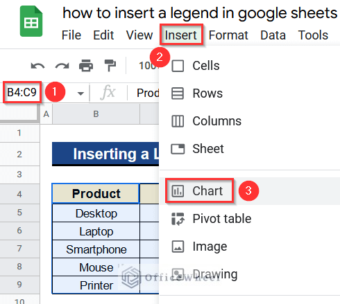
• Firstly, activate all the cells of your dataset from Cell B4 to Cell C9.
• Then, go to Insert > Chart to create a chart from the dataset.

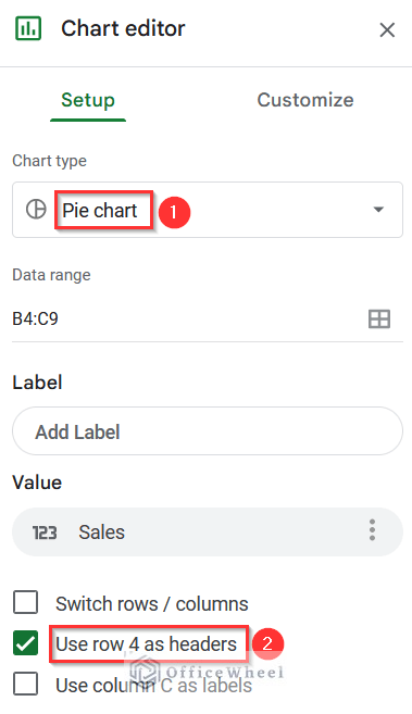
• Next, the Chart Editor window will open.
• Select the Pie Chart option under the Chart Type menu from there. We are choosing this option because we want to make a Pie Chart from our dataset.
• We’ll use Row 4 of our dataset as the header row. Because the headers of our values are in Row 4 of the dataset.
• So, give a tick beside the option Use Row 4 As Headers. Google Sheets is automatically considering Row 4 of our dataset as Header.

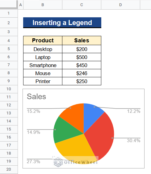
• At last, the Pie Chart will be created with the sales percentage of every product.
• Now, we have to insert a legend in our Pie Chart.

Read More: How to Insert Error Bars in Google Sheets (3 Practical Examples)

Step 2. Open Chart Editor

We have to open the Chart Editor window to insert a legend on our Pie Chart in Google Sheets. We have the sales percentage of every product in our Pie Chart. But we don’t know which percentage is representing which product. That’s why we have to insert a product name as a legend on our Pie Chart. You’ll find the process below:

• At first, Double-Click on any of the values of the Pie Chart, here 12.2% by using the mouse to open the Chart Editor window.

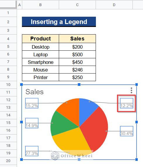
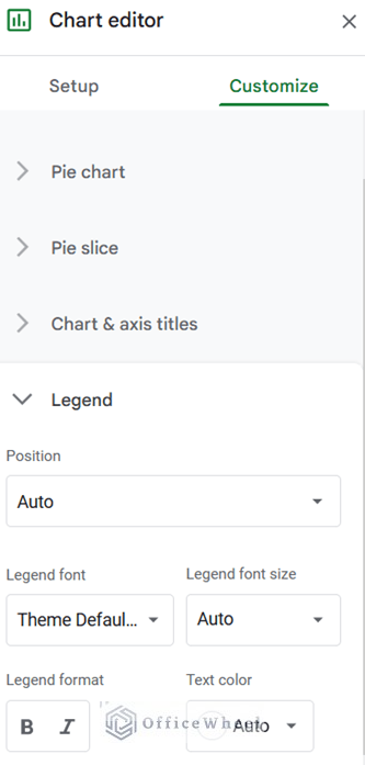
• Then, you’ll see the Chart Editor window where you can find a menu called Legend.
• In the next step, we’ll change the text label to insert a legend in our Pie Chart.

Read More: How to Insert Sparklines in Google Sheets (4 Useful Examples)

Step 3. Change Text Label

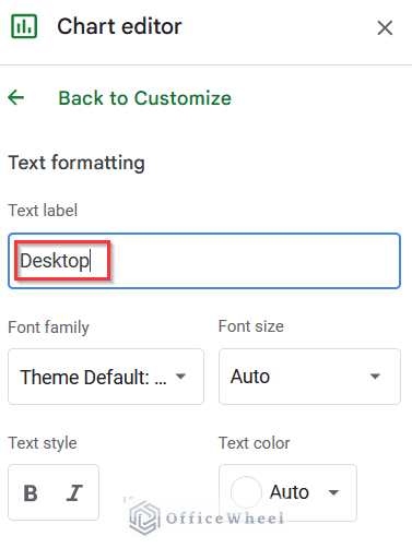
We are going to insert the product titled “Desktop” as a legend on our Pie Chart. So we have to change the text label by opening the Chart Editor window. Let’s see how to do it.

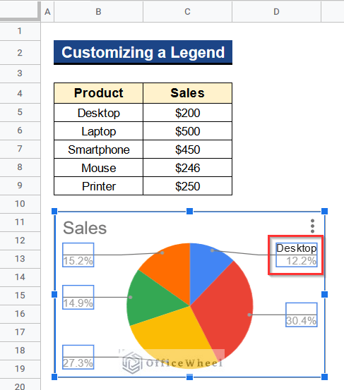
• Again, to open the Chart Editor window, use the mouse to Double-Click on the 12.2% of the Pie Chart.
• We are clicking on the 12.2% because we’ll insert a legend here, which is a product titled “Desktop”.

• Then, you’ll reach at Chart Editor window.
• Next, type “Desktop” in the text box under the Text Label menu and hit Enter.

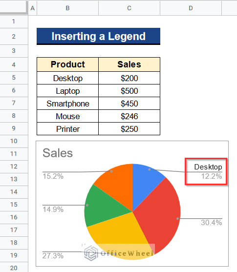
• Finally, you’ll see the legend “Desktop” on the Pie Chart of your Google Sheets.

By following this way, you can easily add each legend individually.

Similar Readings

• How to Insert a Textbox in Google Sheets (An Easy Guide)
• Insert Rows Between Other Rows in Google Sheets (4 Easy Ways)
• How to Insert Multiple Rows in Google Sheets (4 Ways)
• Insert Page Break in Google Sheets (An Easy Guide)
• How to Have More than 26 Columns in Google Sheets

How to Customize a Legend in Google Sheets

In the previous part, we have known about the step-by-step process of how to insert a legend in Google Sheets. But sometimes we need to customize the legend we insert in our chart. There are options for customizing a legend in Google Sheets also. We can change its position, format it, and edit the text label into another text conveniently. The methods are shown below.

1. Changing Position of a Legend

We can change the position of a legend on any chart in Google Sheets. By default, you’ll see your legend on the right or left side of your chart. You can bring it to the top or bottom or any other place you wish on your chart. The process is very simple.

Steps:

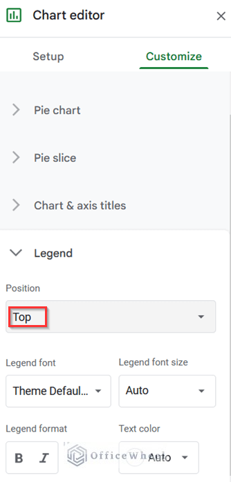
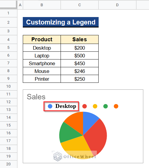
• Before all, to launch the Chart Editor window, Double-Click on the legend “Desktop” on the Pie Chart in your Google Sheets.

• Then, choose the position as Top from the Legend menu under the Chart Editor window because we want to change the position of the legend “Desktop” from side to top.
• You can pick any position you like from this Legend menu.

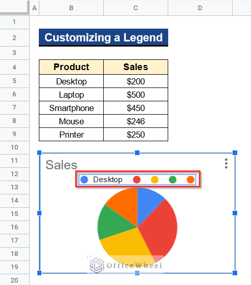
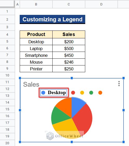
• In the end, we can see the legend placed at the top position of the Pie Chart.

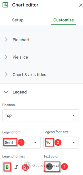
2. Formatting the Legend

We can also format the legend on the chart. You could change the Font Type, Font Size, and Text Color of the legend quickly from the Chart Editor window. We format a legend to make it simple for the eyes to see.

Steps:

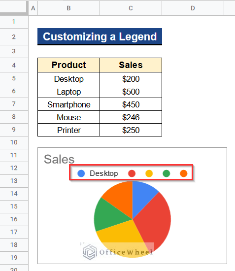
• Initially, to access the Chart Editor window, Double-Click the word “Desktop” on the Google Sheets Pie Chart.

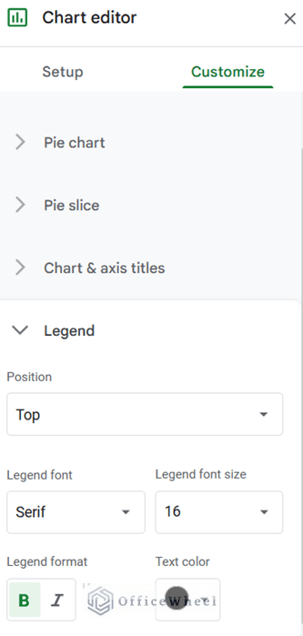
• Here you can choose the Font Type, Font Size, Format, and Text Color under the Legend menu.
• We choose Serif as the Font Type and 16 as the Font Size.
• We also make the Text Format Bold and the Text Color Black.

• Ultimately, you’ll find the formatted legend at the top of the Pie Chart.

3. Editing Text of a Legend

Suppose, we have interred a false legend on our Pie Chart. We want to label our legend as “Laptop” but instead, we label it as “Desktop”. You can edit this legend quickly from the Chart Editor window. Below you’ll find the steps.

Steps:

• First and foremost, Double-Click the word “Desktop” on the Google Sheets Pie Chart by using the mouse.

• You’ll reach the Chart Editor window.

• Again, Double-Click on the word “Desktop” to open the Text Formatting menu.

• After that, type “Laptop” in the text box to change the legend from “Desktop” to “Laptop”.
• Next, press Enter to change the legend.

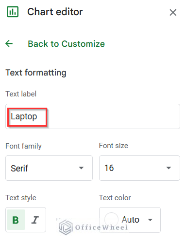
• Finally, the legend will change from “Desktop” to “Laptop” on the Google Sheets Pie Chart.

Conclusion

That’s all for now. Thank you for reading this article. In this article, I have discussed the step-by-step process of how to insert a legend in Google Sheets. I have also discussed how to customize a legend in Google Sheets. Please comment in the comment section if you have any queries about this article. You will also find different articles related to google sheets on our officewheel.com. Visit the site and explore more.

Related Articles

• How to Insert Superscript in Google Sheets (2 Simple Ways)
• Insert Button in Google Sheets (5 Quick Steps)
• How to Add Parentheses in Google Sheets (5 Ideal Scenarios)
• Insert Formula in Google Sheets for Entire Column
• How to Insert Equation in Google Sheets (4 Tricky Ways)
• Insert Video in Google Sheets (2 Easy Ways)
• How to Insert a Header in Google Sheets (2 Simple Scenarios)