How to Insert a Calendar in Google Sheets (2 Effective Ways)

We often require a calendar in Google Sheets to organize our tasks. Having a calendar in Google Sheets can be of great use to track an in-house marketing campaign, categorize a client’s upcoming projects, or allocate an event calendar with pivotal stakeholders. In this article, I’ll demonstrate 2 effective ways of how to insert a calendar in Google Sheets. I’ll also show an easy method to insert a date picker in Google Sheets. The following is an overview of the required output.

Table of Contents

A Sample of Practice Spreadsheet

You can copy our practice spreadsheets by clicking on the following links. The spreadsheets contain an overview of the datasheet and an outline of how to insert a calendar.

Creating Calendar Manually

Inserting Calendar from Templates

2 Effective Ways to Insert a Calendar in Google Sheets

There are 2 feasible ways to insert a calendar in Google Sheets. One of these is to create a calendar manually and another one is to insert a calendar from the Google Sheets templates. Now, let’s start.

1. Creating Calendar Manually

It’s unfortunate to not have any default function or built-in macro to automate the process of inserting a calendar. However, you can follow the steps discussed below to minimize the tedious process and manually insert a calendar efficiently.

Steps:

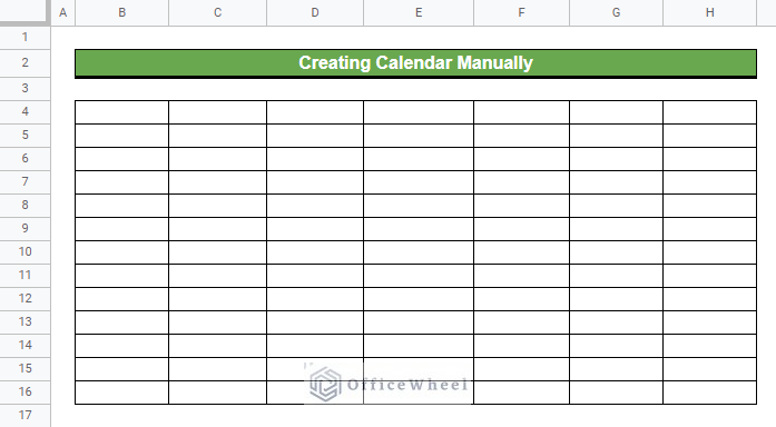
Firstly, take a dataset like the following in Google Sheets.

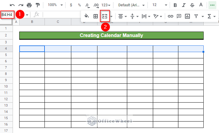
Afterward, select the range B4:H4 and click on the Merge Cells feature.

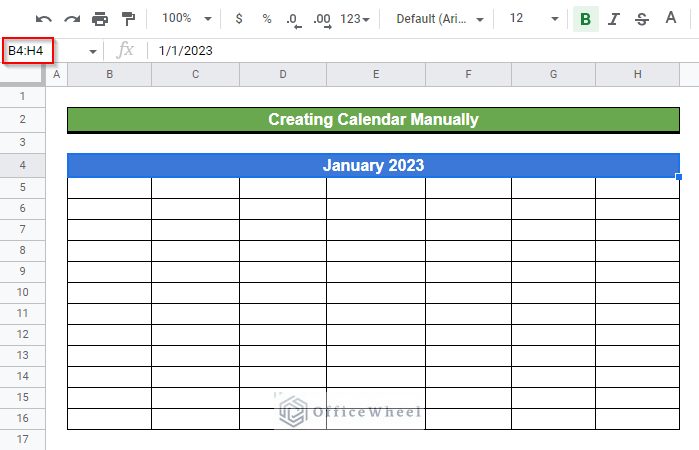
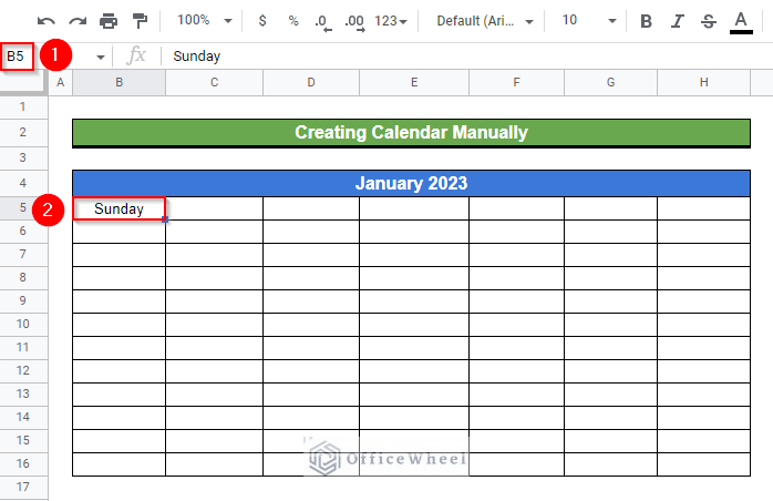
Now, enter the text “January 2023” in the merged cell and format the merged cell with your preferred Fill Color, Text Color, and Text Format.

Now, we have to enter the weekday titles. For that, first, activate Cell B5 by double-clicking on it and then enter the word “Sunday”. Here, we are following the American style. You can follow your preferred style.

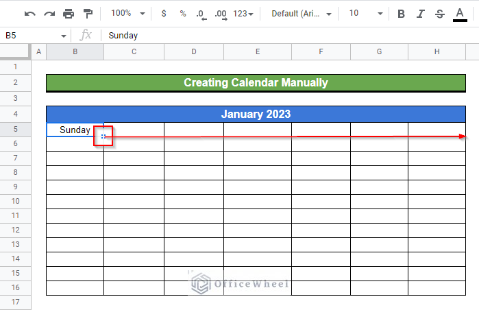
Now, hover your mouse pointer above the bottom-right corner of the selected cell. The Fill Handle icon will be visible at this point.
Use the Fill Handle icon to replenish other cells of Row 5.

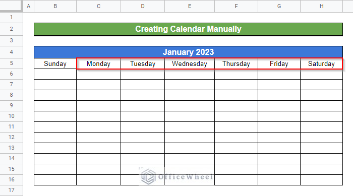
Thus, we have all the weekday titles.

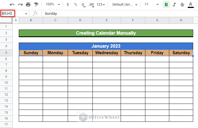
Now, format the range B5:H5 with your preferred Fill Color, Text Color, and Text Format.

Consequently, we have to insert the dates now. For the starting date, first, double-click on the merged Cell B4:H4.
A calendar for the January month of the year 2023 will pop up. As we can see the 1st of January is on Sunday, we’ll enter this date in the column of Sunday.

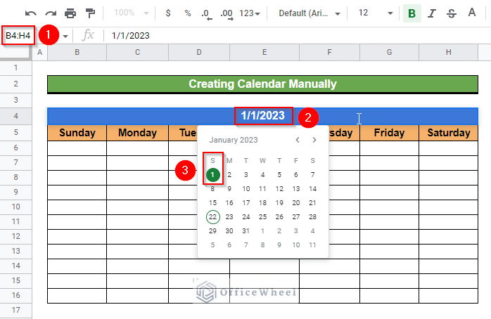
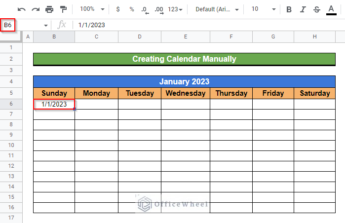
Hence, select Cell B6 and enter the date “1/1/2023”. The date format here is in American style i.e. Month/Day/Year.

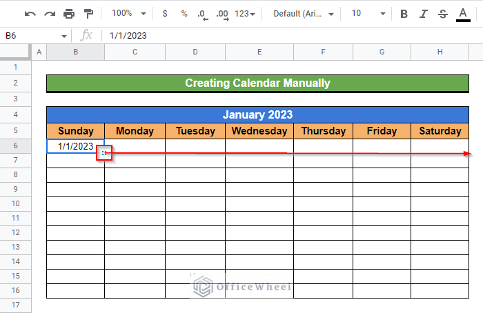
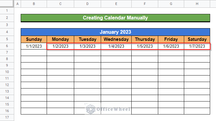
Again, use the Fill Handle icon to replenish the dates in other cells of Row 6.

Now, we have dates for the first week of January month. Now, we’ll keep a row empty because we might want to insert keynotes for a day there.

Therefore, select Cell B8 and enter the date 1/8/2023.

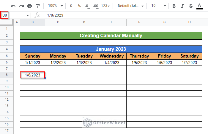
Use the Fill Handle icon to replenish other cells of Row 8.

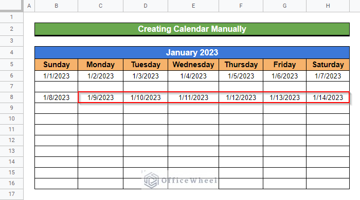
Continue this process for the rest of the days of January month.

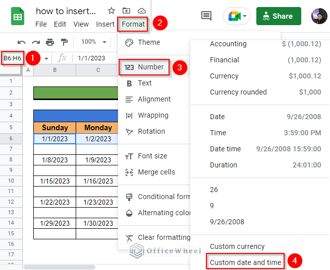
Now, some of us might want to show only the “Day” instead of the “Month/Day/Year” format since the month name and year number are mentioned in the topmost cell of the data table.
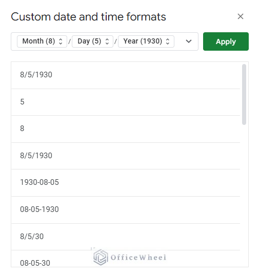
Therefore, to show only the Day information despite keeping the date formatting, go to the Format ribbon and from the appeared options, first, select the Number option and then click on the Custom Date and Time feature.

A pop-up window like the following with appear.

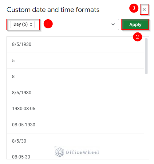
Now, delete the Month and Year Afterward, click on the Apply command and close the window.

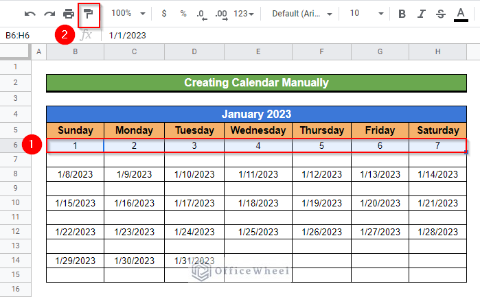
As you can see, the dates are formatted with the required custom format. Now, to copy the format to other dates, we’ll use the Paint Format feature.
While selecting the range B6:H6, click on the Paint Format feature.

Now, select the range B8:H8 to paste the copied format.

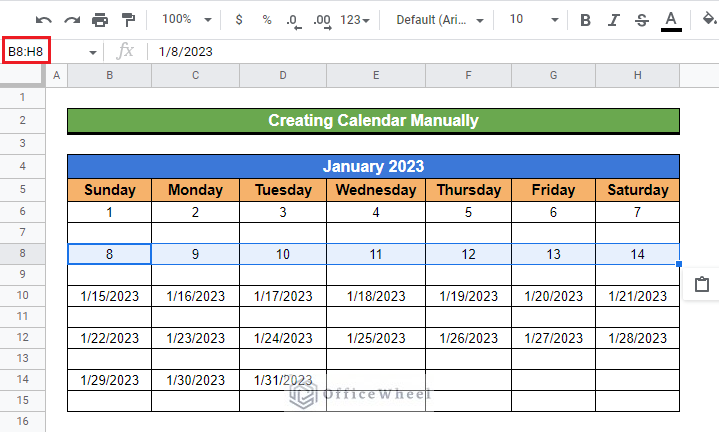
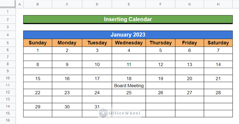
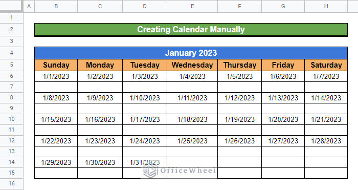
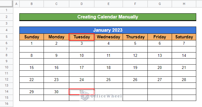
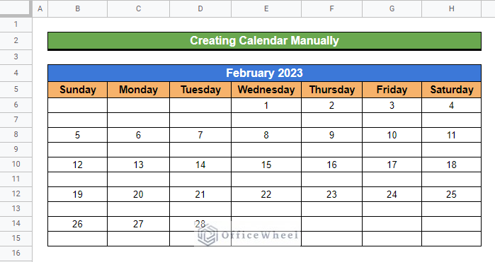
Continue this process for other rows as well. The final output for the January month calendar looks like the following.
Also, not that the final date of January 2023 is Tuesday. Therefore, the first date of February 2023 must be Wednesday.

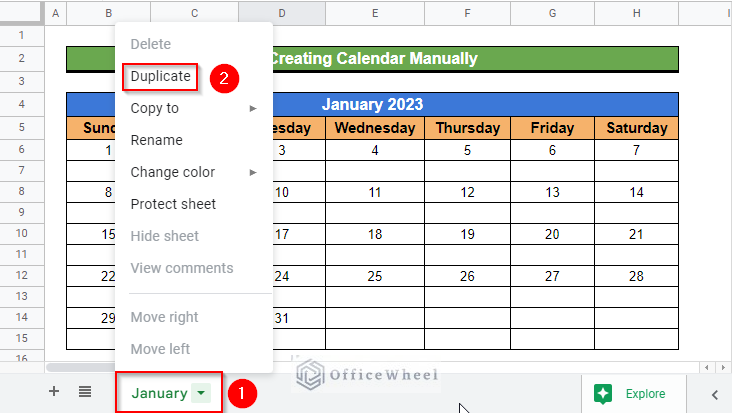
Now, rename the Worksheet to January, and consequently, right-click on the mouse to open a list of options like below. Select the “Duplicate” command from the list.

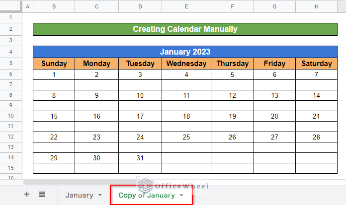
A copy of the first worksheet has been created. This will reduce the amount of work for formatting the calendar for February month.

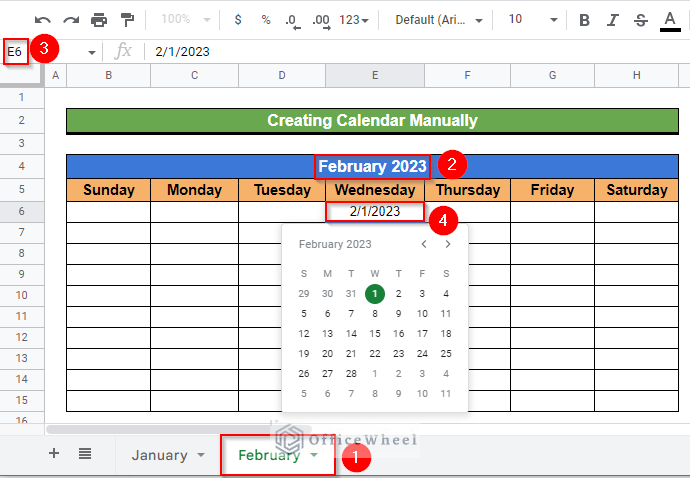
Now, rename the month to February 2023.
Afterward, clear all the values and then, insert the first date of February, e. 2/1/2023 in Cell C6 (column of Wednesday).

Now, follow the steps used for January month to replenish the remaining cells for February 2023.

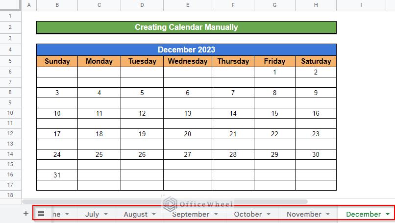
And lastly, copy these methods for creating a calendar for the remaining months of 2023.

2. Inserting from Google Sheets Template Gallery

If creating a calendar manually seems too tedious, you can insert a calendar from existing Google Sheets templates. Follow these simple steps to insert a calendar from Google Sheets templates.

Steps:

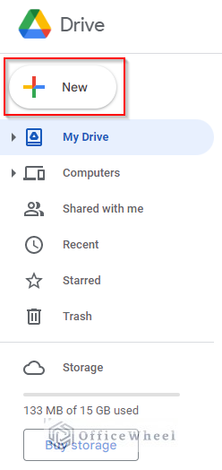
First, open Google Drive from your browser.
Afterward, click on the New command.

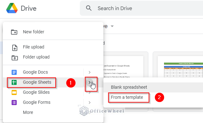
From the appeared list, first, select Google Sheets and then click on From a Template command.

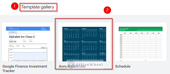
At this time, the Template Gallery should appear. Select the Annual Calendar template from Template Gallery.

Consequently, a Google Sheets file with an annual calendar like the following will open.

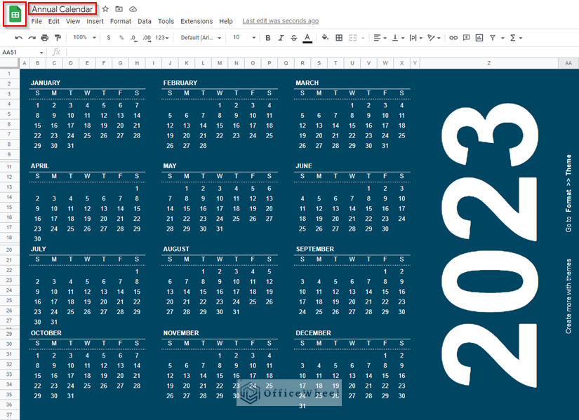
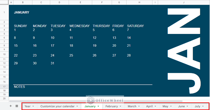
Along with the annual calendar, individual monthly calendars are also present in the Google Sheets file.

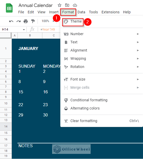
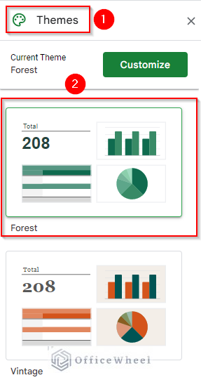
Now, if you require to change the theme of any worksheet, then, go to the Format ribbon and select the Theme option.

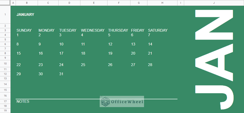
At this point, a sidebar like the following will appear. Select your preferred theme. I’ll select the Forest theme here.

After selecting the Forest theme, the calendar now looks like the following.

How to Insert a Date Picker in Google Sheets

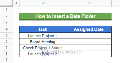
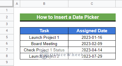
Another frequently used tool in Google Sheets is a date picker. Here, we’ll discuss the process of inserting a date picker with Data Validation in Google Sheets. Let’s have a look at the following dataset. We have a list of tasks here. We want to insert date pickers for these tasks. Now, let’s start.

Steps:

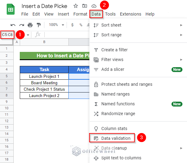
To start, select range C5:C8 first and then go to the Data ribbon.
Select the Data Validation feature from the appeared list of options.

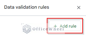
A sidebar like the following will appear. Click on the +Add Rule command.

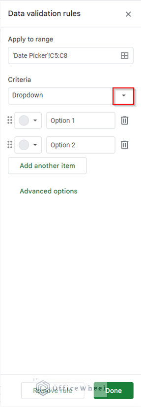
Consequently, the sidebar will change like the following. Click on the drop-down icon of the Dropdown Criteria.

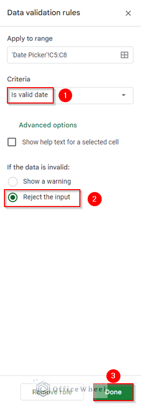
From the drop-down list, select the Is Valid Date The sidebar has now changed to the following format.
Now, select the Reject the Input option for invalid dates.
Lastly, click on Done.

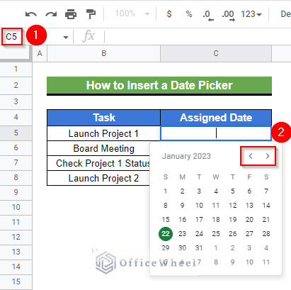
At this time, double-click on Cell C5, and a date picker will pop up.
Use the “<” and “>” icons for moving to the previous and next month respectively.
Finally, pick your required date from the pop-up calendar.

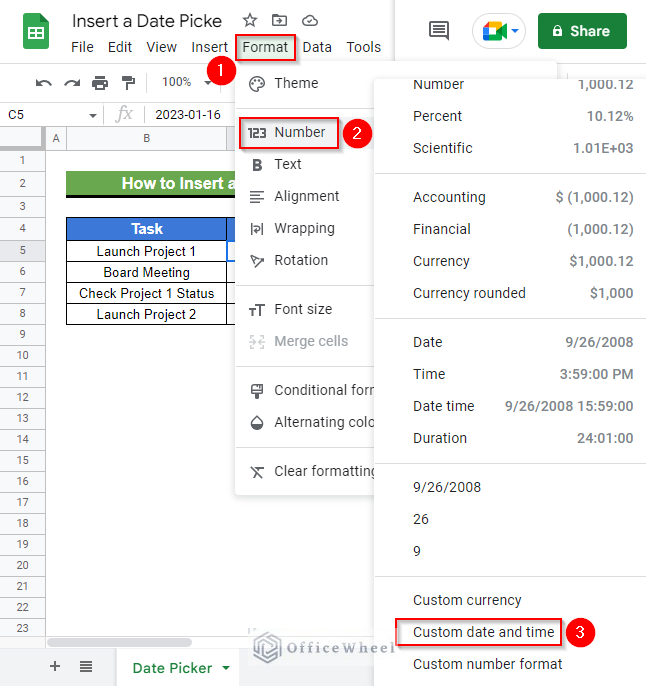
If you require changing the formatting of the date, you can change that from the Custom Date and Time feature which is available in the Format ribbon under the Number option.

Now, similarly, pick a date for the rest of the tasks. The final output looks like the following.

Conclusion

This concludes our article to learn how to insert a calendar in Google Sheets. I hope the demonstrated examples were ideal for your requirements. Feel free to leave your thoughts on the article in the comment box. Visit our website OfficeWheel.com for more helpful articles.

How to Insert a Calendar in Google Sheets (2 Effective Ways)

A Sample of Practice Spreadsheet

2 Effective Ways to Insert a Calendar in Google Sheets

1. Creating Calendar Manually

2. Inserting from Google Sheets Template Gallery

How to Insert a Date Picker in Google Sheets

Conclusion

Related Articles

Seemanto Saha

Leave a reply Cancel reply