How to Make a Tournament Bracket in Google Sheets (Easy Steps)

Using Google Sheets to create a tournament bracket is an efficient way to track a competition’s progression, whether for sports or personal use. The process is straightforward and can be completed in several steps. In this article, we will discuss how to make a tournament bracket in Google Sheets.

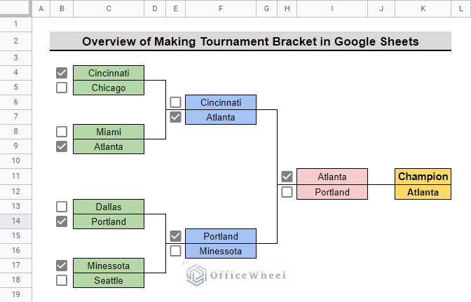
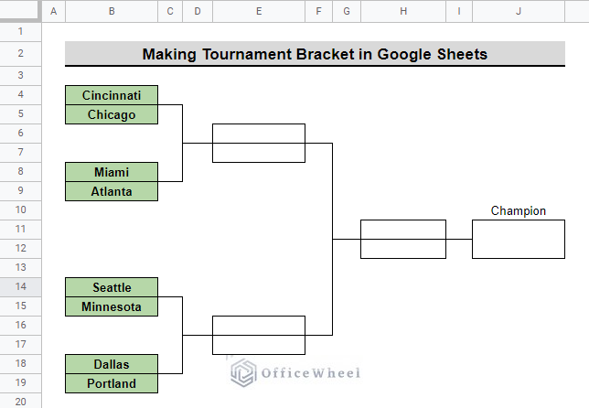
The above screenshot is an overview of the article, representing how to make a tournament bracket in Google Sheets.

Table of Contents

A Sample of Practice Spreadsheet

You can download the spreadsheet and practice the techniques by working on it.

Making Tournament Bracket

Step-by-Step Process to Make Tournament Bracket in Google Sheets

We will show you how to make a tournament bracket with 8 teams in Google Sheets. Follow the below steps.

Step 1: Create Dataset

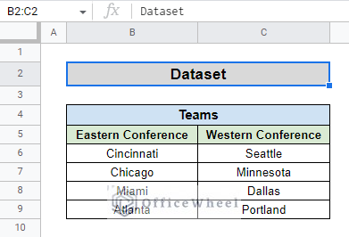
We will use the following dataset to make a tournament bracket comprising 8 teams:

The dataset has 8 teams from Major League Soccer (MLS).
4 teams are from the Eastern Conference and the other 4 teams are from the Western Conference.

Step 2: Bracket Selection

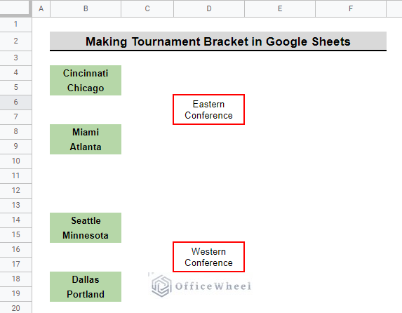
To make a tournament bracket we must first have two sides or brackets.

The two brackets will comprise 4 teams each. We place the teams from the Eastern Conference in one side or bracket and place the teams from the Western Conference in another side or bracket.

Step 3: Selecting Border

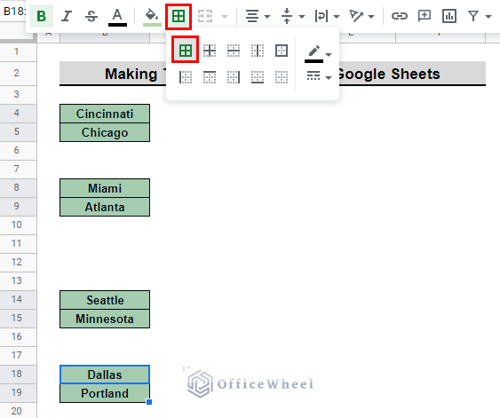
Go to Menu > Borders to select the border that you want the teams to have. We select All borders for all of the teams in our example.

Similar Readings

Step 4: Making Progress Lines

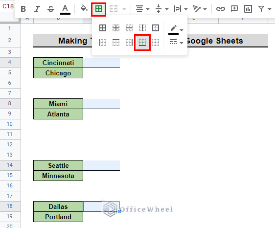
Progress lines show who wins a matchup and will progress to the next round in the tournament. The matchup between Cincinnati and Chicago will have a winner and the winning team will progress to the next round.

First, select the top cells adjacent to each pair of teams and select the Bottom border from the Borders menu.

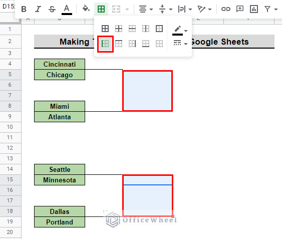
After that, select the cells between the newly created bottom borders and select the Left border from the Borders menu.

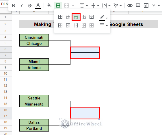
Then, select the two middle cells and select the Horizontal borders from the Borders menu.

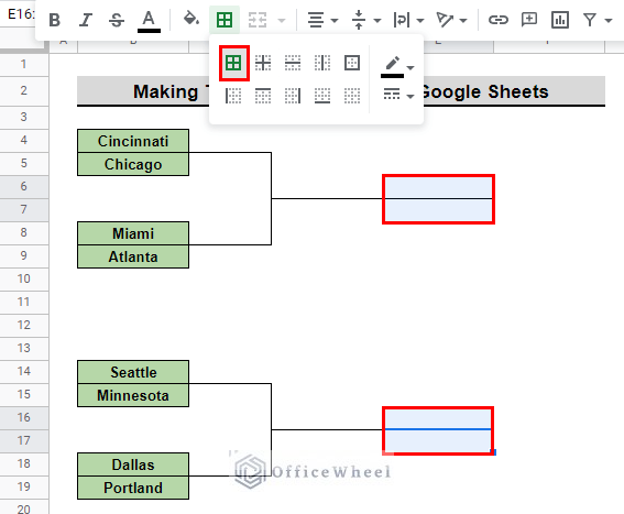
Afterward, select two cells adjacent to the newly created Horizontal border and select all borders to create a box for the winning teams.

Step 5: Completing the Bracket

Repeat Step 4 to complete the tournament bracket.

Similar Readings

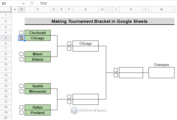
Step 6: Adding Checkboxes

Checkboxes can be added with the IFERROR and VLOOKUP functions to make the tournament bracket more interactive and attractive.

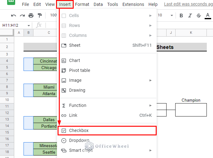
First, insert a column before the team names and insert checkboxes in these cells by selecting these cells and going to Menu bar > Insert > Checkbox.

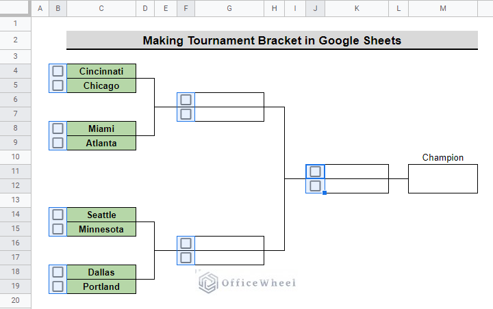
This is how the tournament bracket looks after inserting checkboxes.

After that, type the following formula in the second matchup cell.

=IFERROR(VLOOKUP(TRUE,B4:C5,2,FALSE),"")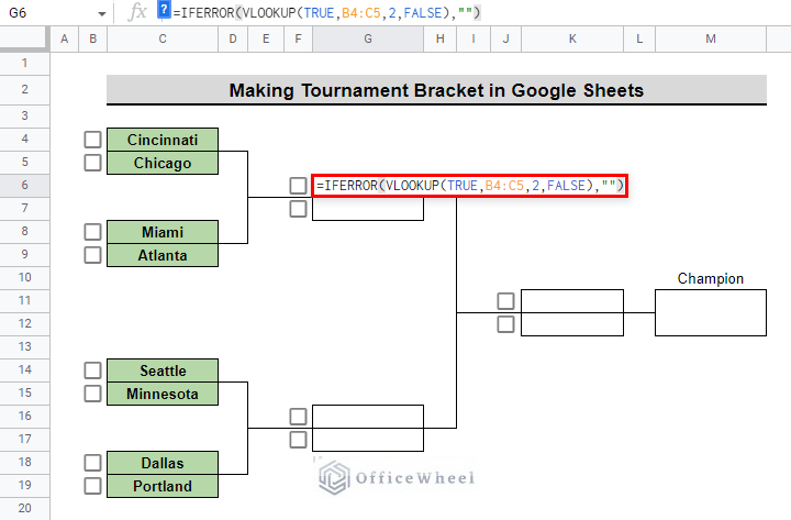

Formula Explanation:

VLOOKUP(TRUE,B4:C5,2,FALSE)

VLOOKUP will look for TRUE (checkbox result) in the B4:C5 range, which represents the two competing teams.
The value 2 in the formula allows it to return the value from the 2nd column of the range if it finds a match, in other words, the winning team.

IFERROR(VLOOKUP(TRUE,B4:C5,2,FALSE),””)

IFERROR will return a blank cell if VLOOKUP does not find a match.

This formula will allow us to select which team progresses to the next round without having to type the team name over and over again. If the team progresses to the next round, just check the boxes.
A similar formula is applied to every winning bracket cell until the Champion bracket.

Step 7: Finalizing Tournament Bracket

We use custom formatting for the cells to complete the tournament bracket.

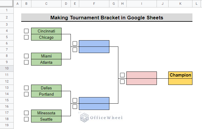
This is how the final tournament looks after getting a champion.

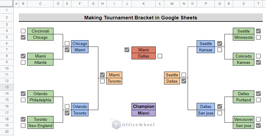
Note: We can even make a tournament bracket for 16, 32, and 64 teams in this way.

Below is an example of making a tournament bracket that consists of 16 teams.

Conclusion

This article demonstrates the ways to make a tournament bracket in Google Sheets. We recommend you practice the techniques to understand them fully. The goal of this article is to provide helpful information and guide you in completing your task.

Additionally, consider looking into other articles available on OfficeWheel to expand your understanding and skill in using Google Sheets.