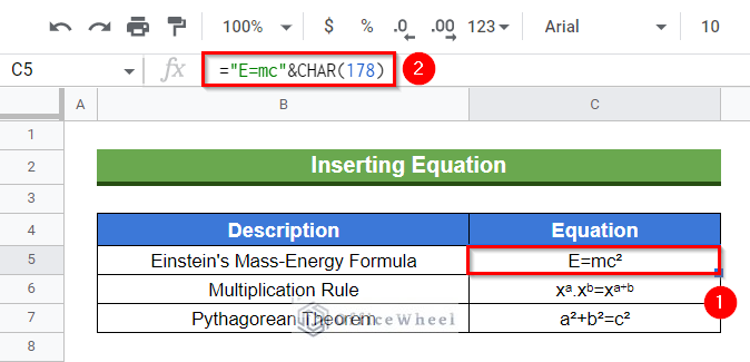
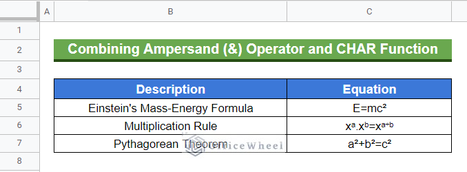
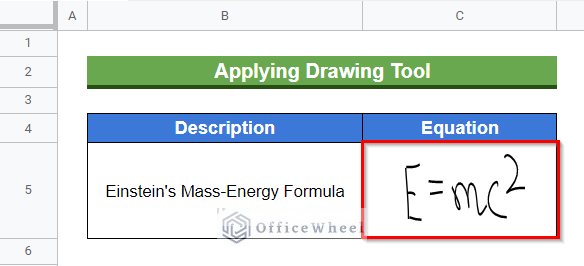
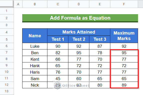
How to Insert Equation in Google Sheets (4 Tricky Ways)

Equations are often used in our calculations to express a precise and quantitative relationship between various features of our world. Since we heavily use Google Sheets in our day-to-day life, it is apparent that we’ll require inserting equations in Google Sheets. However, unlike Google Docs, we don’t have any built-in feature to insert equations in Google Sheets. In spite of that, I’ll show you 4 easy ways to insert an equation in Google Sheets. The following image contains an overview of the required output. Here, I have inserted a simple equation by applying a formula. Now, let’s learn the ways.

Table of Contents

A Sample of Practice Spreadsheet

You can copy our practice spreadsheet by clicking on the following link. The spreadsheet here contains an overview of the demonstrated ways to insert an equation in Google Sheets.

Inserting Equation

4 Tricky Ways to Insert Equation in Google Sheets

Here, we’ll use operators, built-in features, and formulas to insert an equation in Google Sheets. Since Google Docs has an in-house feature to insert equations, we’ll also seek help from it. Now, let’s start.

1. Combining Ampersand (&) Operator and CHAR Function

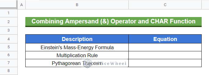
Our first method will use a combination of the Ampersand (&) operator and the CHAR function. The CHAR function is able to convert a number into a character. One limitation of this method is that complex equations that contain fractions or any mathematical operators (for example, the Summation, Differential, Integral, etc. operators) can’t be inserted with this method. Now, let’s have a look at the dataset we’ll use for this method. The dataset contains a list of famous formulas for which we’ll write the related equation.

Steps:

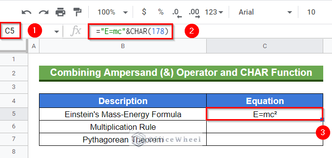
Initially, activate Cell C5 by double-clicking on it.
Afterward, type in the following formula-

="E=mc"&CHAR(178)

Then, press Enter key to get the required output. Here, the statement CHAR (178) converts the decimal code 178 to superscript 2.

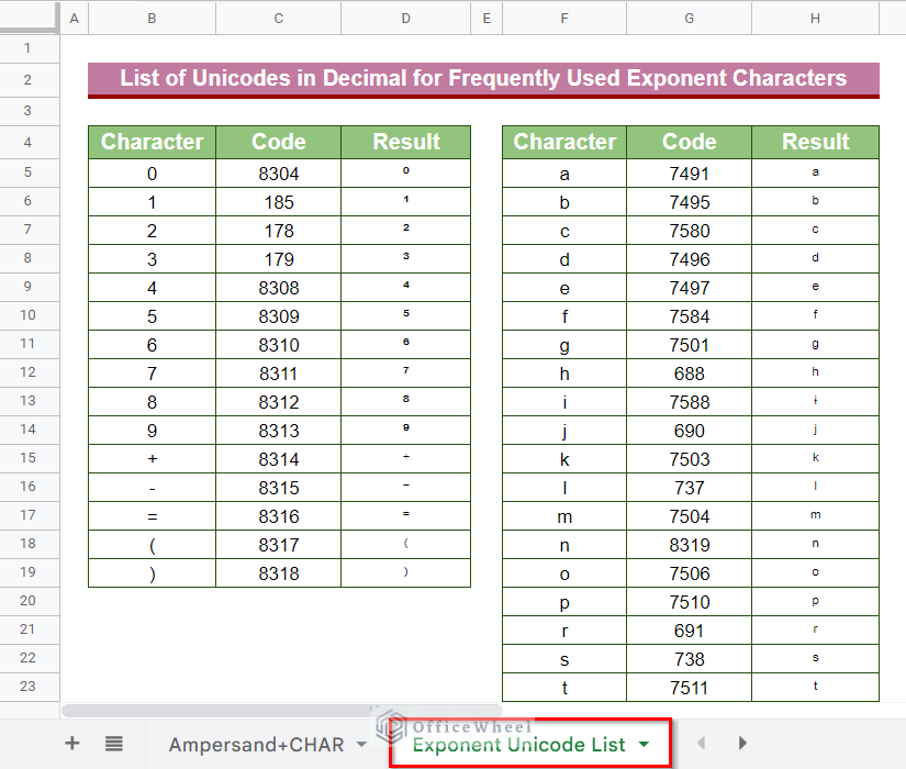
We need a list of codes for inserting the equations in the remaining cells. Such a list is provided in the worksheet titled “Exponent Unicode List”. Use the required codes from here and complete the formula in other cells.

The final output looks like the following-

2. Applying Drawing Tool

In this method, we’ll use the in-house feature of inserting drawings in Google Sheets. We can insert an equation as hand-scribbled text through the Drawing tool in Google Sheets. Keep reading to learn how.

Steps:

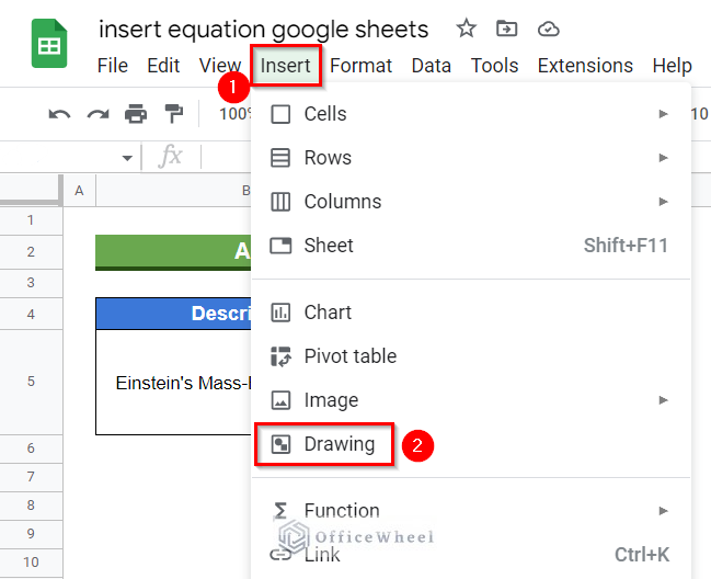
Firstly, go to the Insert ribbon and select the Drawing tool from the pop-up list.

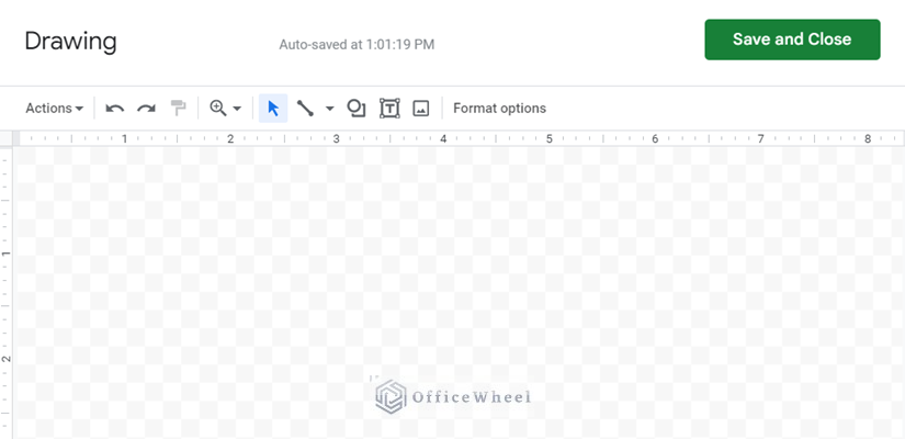
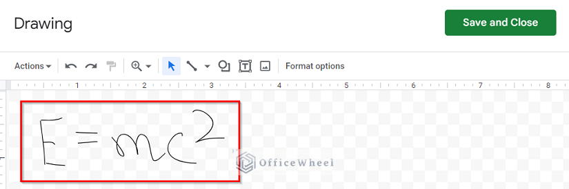
Consequently, a window like the following will pop up.

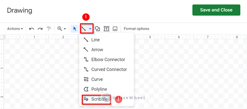
Now, click on the drop-down icon of the Line feature and select the Scribble option from the pop-up list.

Afterward, draw the required equation using the mouse or any external device.

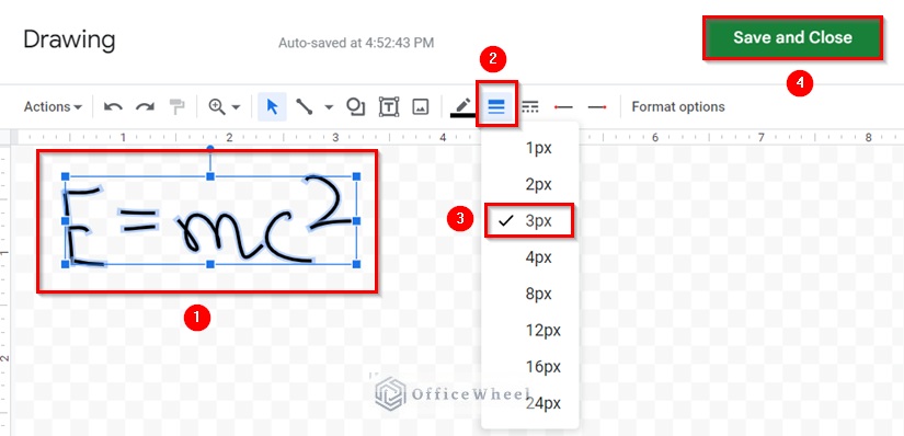
Then, select the entire equation to view the formatting options. Customize the equation with the required formatting options. Here, I have set the Line Weight to 3px.
Now, click on the Save and Close option.

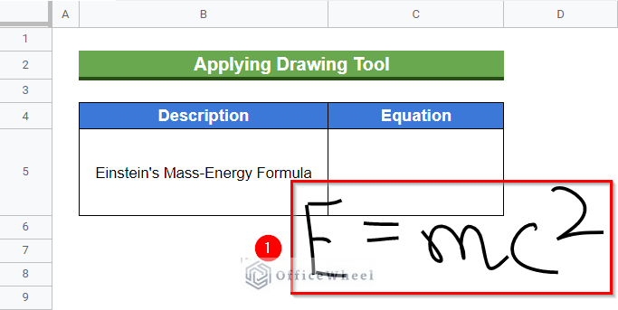
At this point, the hand-scribbled equation will appear in your Google Sheets worksheet.

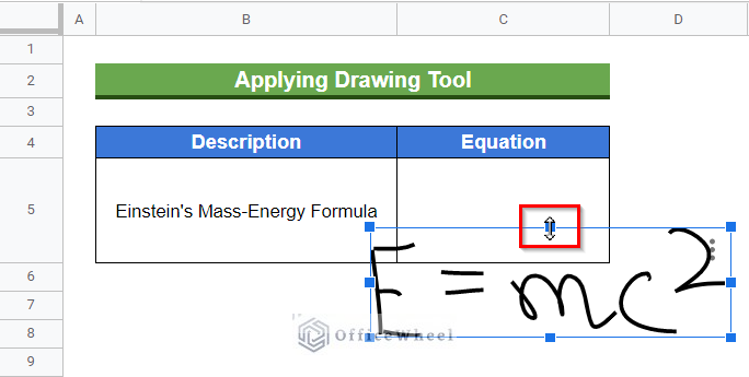
At this time, select the equation and hover your mouse pointer above the square blue icons of the equation border. You will be able to resize the drawing by dragging through this.

Resize the equation and drag it above the required cell to get the required output. One of the limitations of this method is that the inserted equations don’t have aesthetic values.

3. Using Google Docs and Insert Image Option

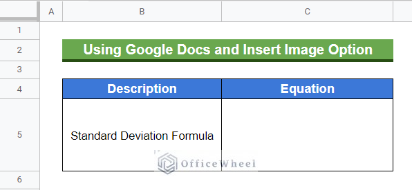
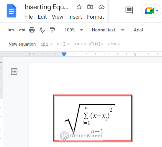
The previously mentioned ways might be able to insert simple equations but to insert equations with various mathematical operators, we need to insert the equation as an image. Since Google Docs has a built-in feature to insert such complex equations, we’ll use Google Docs to write our required equation and then insert the equation as an image. To demonstrate this example, we’ll insert the equation for Standard Deviation Formula in Google Sheets.

Steps:

First, open a Google Docs file.
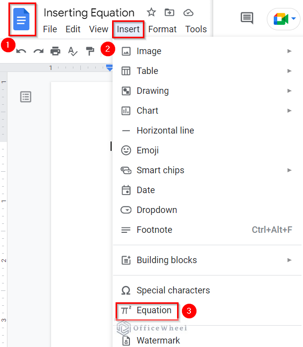
Then, go to the Insert ribbon and select the Equation tool from the appearing list.

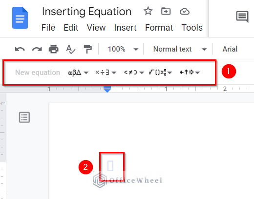
Af this point, the features of the Equation tool and a space for inserting the required equation will appear in your Google Docs file.

Now, use these features to insert the equation for the Standard Deviation formula.

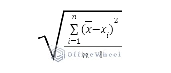
Now, use any Snipping tool to create a screenshot like the following-

Next, we have to insert the screenshot in our Google Sheets file. We can insert the screenshot from our Computer or from Google Drive.

Similar Readings

3.1 Inserting from Computer

Since the screenshot is saved directly on your computer, it’s easier to upload the screenshot from your computer directly. Follow the steps below for this process.

Steps:

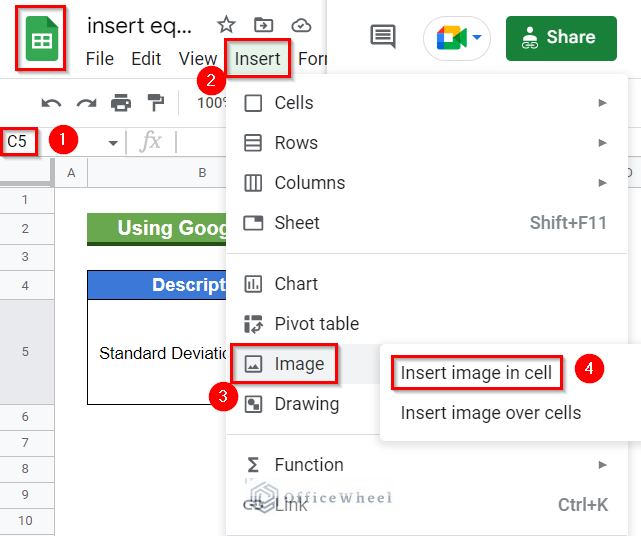
In your Google Sheets, first, select Cell C5 and then go to the Insert ribbon. After that, click on the Image feature. Lastly, select Insert Image in a Cell option from the two options.

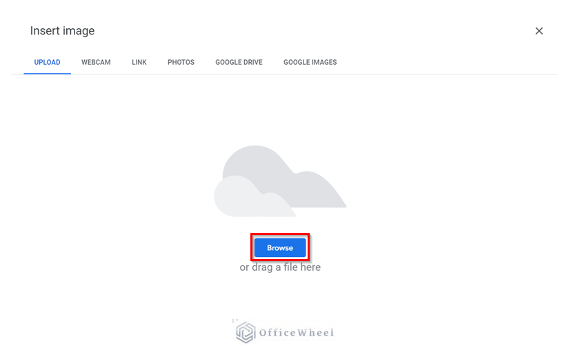
Consequently, a window like the following will pop up. To insert an image from your computer, click on the Browse option. You can also select the required image and drag it above the window to open it.

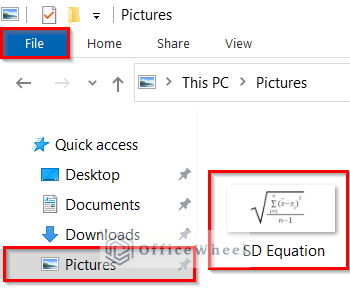
After selecting the Browse option, the File Explorer of your computer will open. Open the folder where you saved the screenshot and double-click on it to open the screenshot into your Google Sheets file.

The final output looks like the following after you insert the image by double-clicking on it.

3.2 Inserting from Google Drive

You can also insert the image from your Google Drive. This option is useful when you are working from a remote computer and you don’t have access to your personal computer. However, the image has to be available in your Google Drive for this method to work.

Steps:

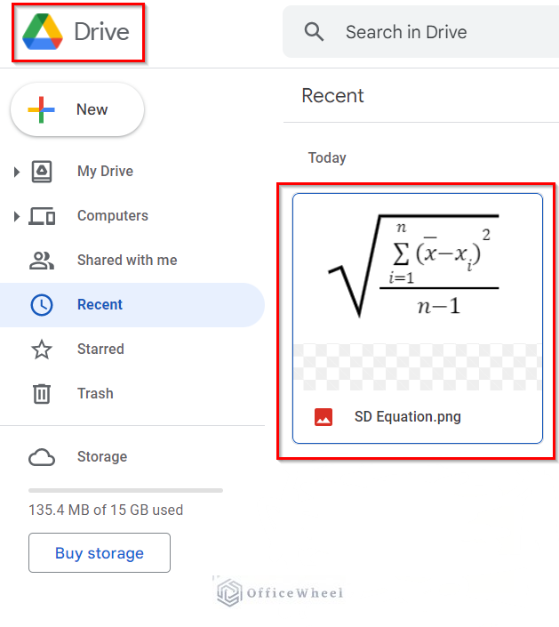
First, upload the screenshot to your Google Drive.

Now, return to your Google Sheets worksheet and select Cell C5.
After that, go to the Insert ribbon first and then click on the Image Lastly, select Insert Image in a Cell option from the two options.

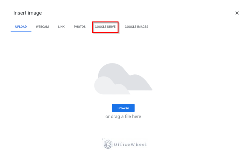
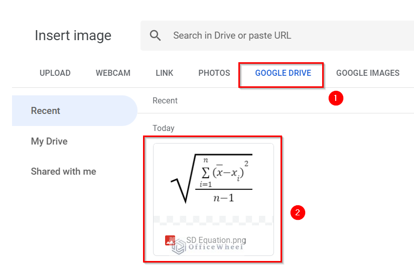
Consequently, a window like the following will pop up. Since we want to insert an image from our Google Drive this time, click on the Google Drive option.

Finally, from your Google Drive files, double-click on the required image to insert it into your Google Sheets.

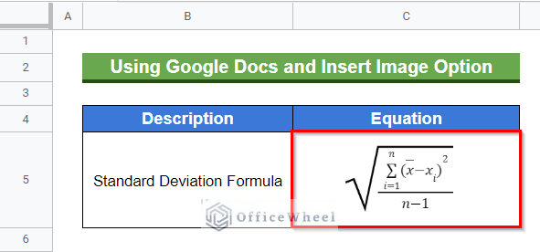
And as you can see, the required equation has appeared in Cell C5.

4. Employing IMAGE Function

We can also insert an image of an equation using the IMAGE function. This function can insert an image in a cell by using the URL of the image as an argument. This method may sound simple, but there are a few important aspects to employing the IMAGE function. Follow the simple steps below.

Steps:

We’ll insert the required image of the equation from Google Drive. Therefore, to get the URL of the image, open your Google drive.
Now, select the image you want to insert.

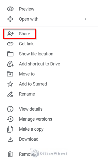
Afterward, right-click with your mouse to pop up a list of options and select the Share command from there.

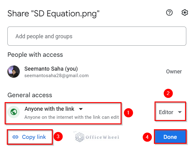
At this time, a window like the following will appear. Set the General Access as Anyone with the Link and the Role as Editor for the proper execution of the formula.
Now, click on the Copy Link option to make a copy of the link first and then click on Done.

However, we have to modify the copied link before using it as an argument for the IMAGE function. Although, this is not required in case the image URL is collected from a Google search.
The link we copied is given below-

https://drive.google.com/file/d/1Sgb0m-LQy49gigJ6Z6t7AO8mtmG5MluN/view?usp=share_link

Change this link to the following-

https://drive.google.com/uc?export=download&id=1Sgb0m-LQy49gigJ6Z6t7AO8mtmG5MluN

Here, we have substituted the “file/d/” part with “uc?export=download&id=” and removed the “/view?usp=sharing” part.
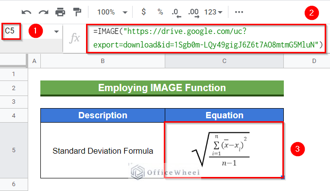
Now, activate Cell C5 by double-clicking on it.
Afterward, insert the following formula-

=IMAGE("https://drive.google.com/uc?export=download&id=1Sgb0m-LQy49gigJ6Z6t7AO8mtmG5MluN")

Finally, get the required output by pressing the Enter key from your keyboard.

Similar Readings

How to Add Equation to Graph in Google Sheets

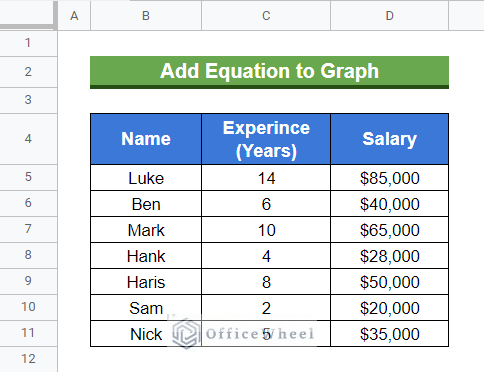
We can also insert an equation to the graph plotted for a dataset in Google Sheets. Let’s have a look at the following dataset. It contains a list of persons’ salary variations with experience. Now, we will plot a graph for this relation and insert an equation for the trendline.

Steps:

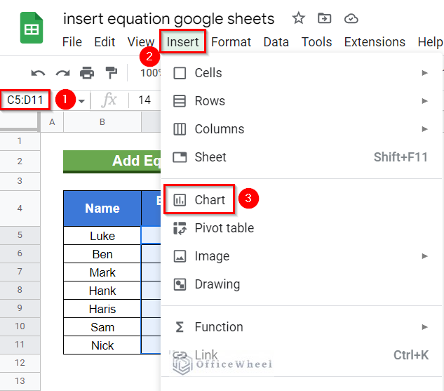
Initially, select the range C5:D11 and then go to the Insert ribbon to select the Chart feature from the appearing list of options.

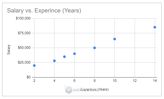
At this point, a Scatter Chart like below will appear.

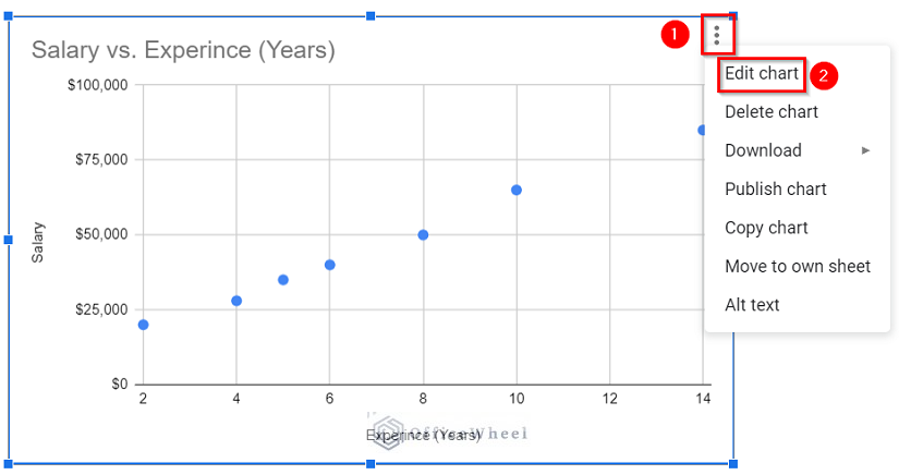
Now, select the chart and click on the vertical ellipsis (⋮) symbol.
Consequently, a list of options will pop up. Select the Edit Chart feature from the list.

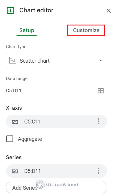
At this time, a sidebar like the following will appear. Go to the Customize menu.

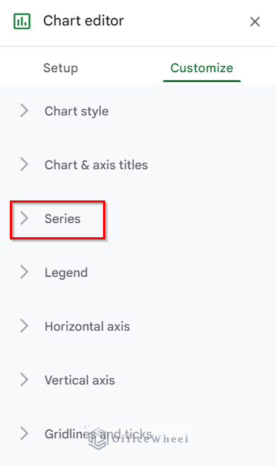
Afterward, select the Series option from Customize menu.

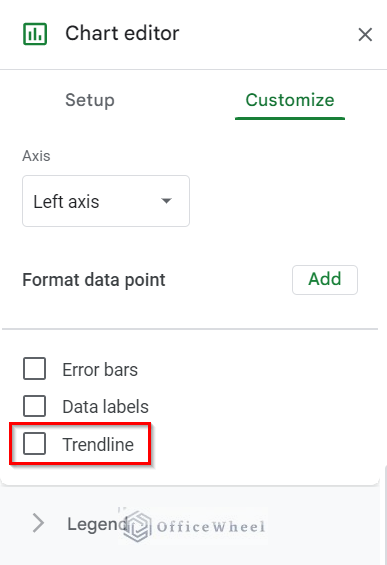
Now, click on the checkbox of Trendline to activate its features.

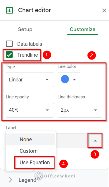
As soon as you check the checkbox of Trendline, a set of features will appear.
You can use the Type, Line Color, Line Opacity, and Line Thickness features to customize the trendline.
Now, click on the drop-down icon of Label and select the Use Equation option from the drop-down list.

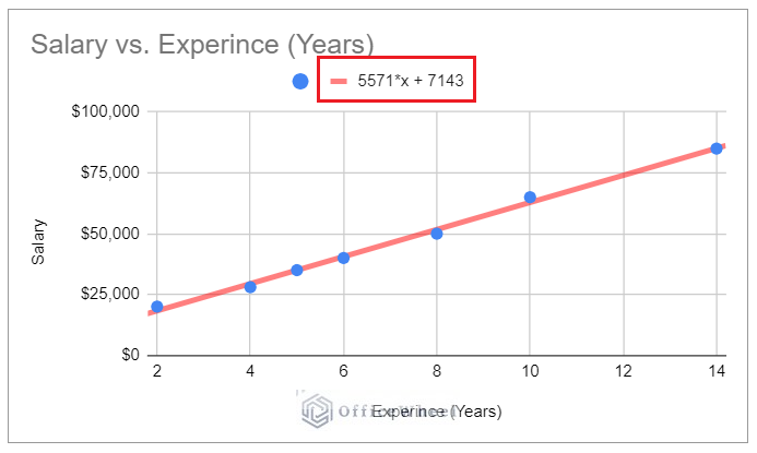
The chart now looks like the following. And as we can see, an equation has been inserted in our chart.

How to Add Formula as Equation in Google Sheets

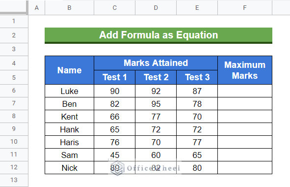
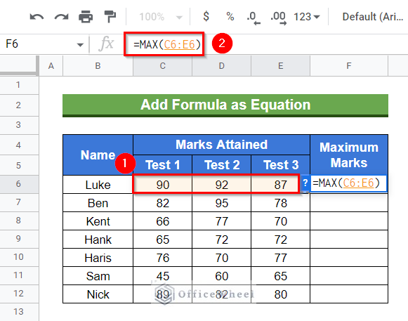
The formulas we use in Google Sheets are also a type of equation. Therefore, let’s learn how to Insert Google Sheets formulas as Equation. Let’s have a look at the dataset below. It contains a list of students’ marks attained in 3 different tests. We want to enumerate the maximum number attained by each student. So, let’s start.

Steps:

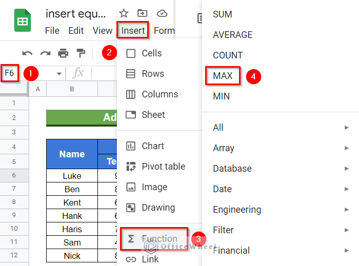
Initially, select Cell F6.
Then, go to the Insert ribbon and select the Function option.
After that, a list of functions will appear. Since we want to enumerate the maximum marks for each student, click on the MAX function.

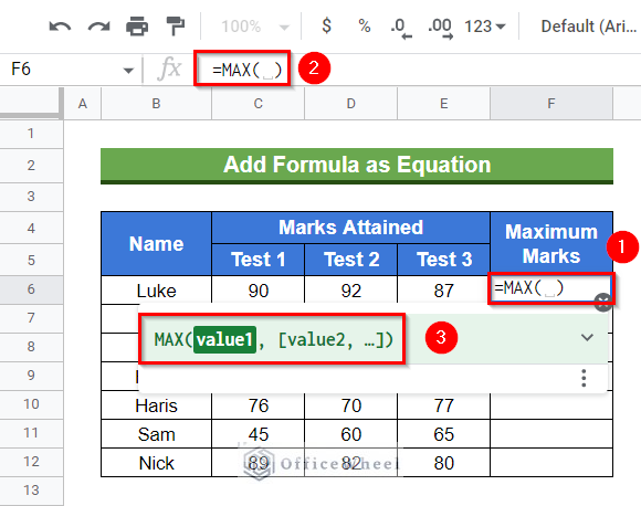
As soon as you click on the MAX option, it will appear on the F6 cell and formula bar. Also, a pop-up of the MAX function with its arguments will appear.

Now, select the range C6:E6 by dragging the mouse pointer over the cells to insert the range as arguments for the MAX function inserted previously.

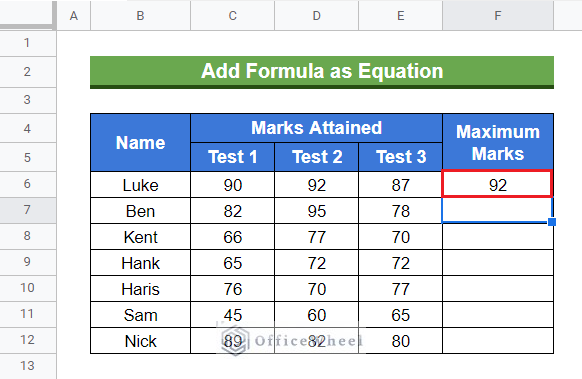
Now, get the required output by pressing the Enter key from your keyboard.

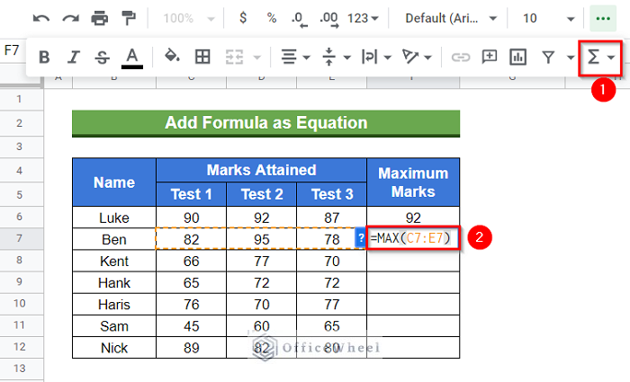
However, we can also insert functions from the Clipboard menu in Google Sheets. Or, we can simply type it in the required cell.

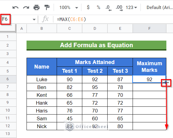
Now, for the rest of the cells, we’ll use the auto-fill feature. For that, select sell F6 again and hover your mouse pointer above the bottom right corner of the selected cell.
At this time, the Fill Handle icon will be visible. Finally, use it to copy the formula to other cells of Column F.

The final output looks like the following. Using these simple steps, you can insert any formula as an equation in Google Sheets.

Things to Be Considered

The Unicode used as an argument for the CHAR function has to be in decimal.
For proper execution of the IMAGE function, we have to set the General Access as Anyone with the Link and the Role as Editor for that image in your Google Drive.
In the case of using images from Google, we can insert the copied URL directly as an argument in the IMAGE However, you have to modify the URL if you are inserting an image from Google Drive.

Conclusion

This concludes our article to learn how we can insert an equation in Google Sheets. I hope the demonstrated examples were ideal for your requirements. Feel free to leave your thoughts on the article in the comment box. Visit our website OfficeWheel.com for more helpful articles.

How to Insert Equation in Google Sheets (4 Tricky Ways)

A Sample of Practice Spreadsheet

4 Tricky Ways to Insert Equation in Google Sheets

1. Combining Ampersand (&) Operator and CHAR Function

2. Applying Drawing Tool

3. Using Google Docs and Insert Image Option

3.1 Inserting from Computer

3.2 Inserting from Google Drive

4. Employing IMAGE Function

How to Add Equation to Graph in Google Sheets

How to Add Formula as Equation in Google Sheets

Things to Be Considered

Conclusion

Related Articles

Seemanto Saha

Leave a reply Cancel reply