Wildcards are a set of special symbols that help you for an effective search result and can represent a group of similar strings at a time. In this article, you will learn about the wildcard in Google Sheets.
A Sample of Practice Spreadsheet
You can download spreadsheets from here and practice.
What Are Wildcards in Google Sheets?
In Google Sheets, Wildcards are advanced search techniques that optimize your searching. The most common wildcard characters in Google Sheets are:
- Question (?): It represents a single character in Google Sheets. For example, ‘T?m’ can refer to Tom, Tim, etc.
- Asterisk (*): It represents any number of characters in Google Sheets. For example, ‘Tom*’ can refer to Tom, Tommy, Tomas, etc.
- Tilde (~): This wildcard character is basically used before* or? wildcards. It instructs Google Sheets to treat these wildcards as a regular symbol. For example, the search term ‘T~*’ means to go for the exact word ‘T*’.
3 Practical Examples of Using Wildcard in Google Sheets
You can use wildcards in different types of functions to get your desired result. Wildcard makes the function more powerful, and the functions are able to present extensive results. the wildcard is mostly used in: SUMIF or COUNTIF function, conditional filtering, and VLOOKUP formulas.
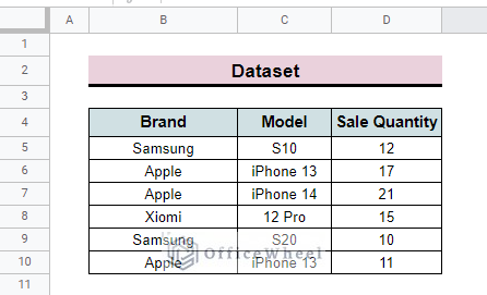
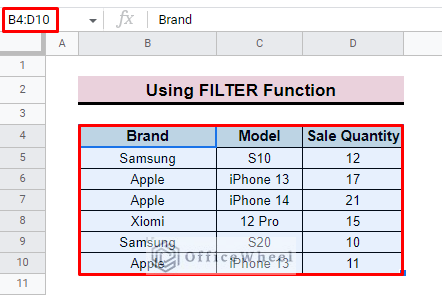
Here, we discuss the use of different types of wildcards with these functions. To show the application of these wildcards we develop a dataset containing mobile phone information. The dataset has Brand, Model, and Sale Quantity columns.
1. Applying Asterisk(*) Wildcard
The asterisk wildcard will help you to look up values that you may not exactly remember. So, you can use this wildcard in a number of functions and can the result that you expect.
1.1 Using SUMIF or COUNTIF Functions
You can use this asterisk wildcard in both SUMIF and COUNTIF functions. To show the whole process here we apply the SUMIF function. You can run the COUNTIF function by following the same procedure.
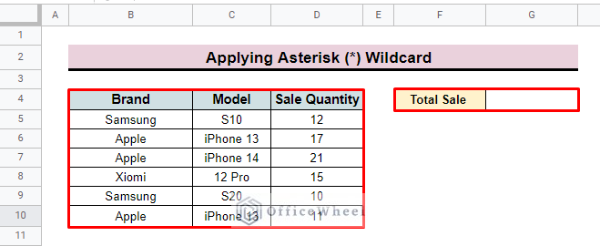
- First, create a row to show the sum result. Here we create a cell Total Sale to show the sale result.
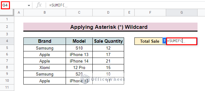
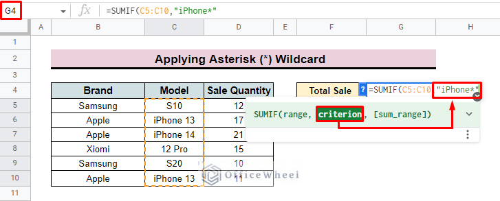
- Then insert the SUMIF function in cell G4.
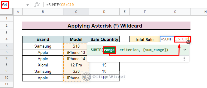
- After that select a range as per the function parameter. Here, we select the entire model column C5:C10 as the range.
- Now, as a criterion argument select a specific value. We add “iPhone*”. Here, with the value, we insert “*” wildcard also to sum all the values that start with “iPhone”.
- At the end, apply the [sum_range] from where sum will be calculated. We insert D5:D10 as the sum range.
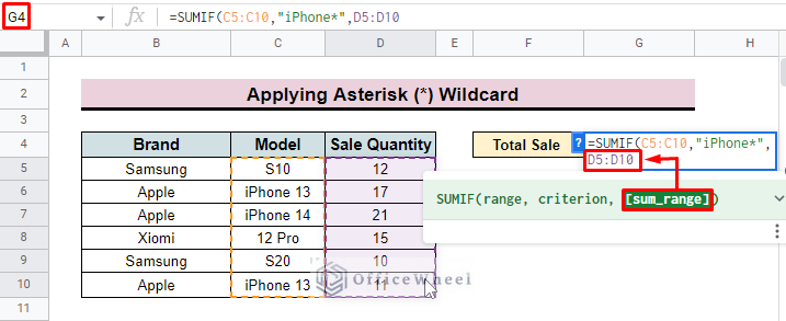
- Finally, press ENTER and find the sum of all iPhone models.
=SUMIF(C5:C10,"iPhone*",D5:D10)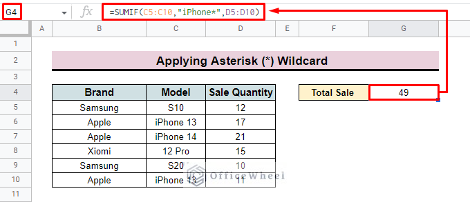
- In the same way, insert the range and criterion for the COUNTIF function.
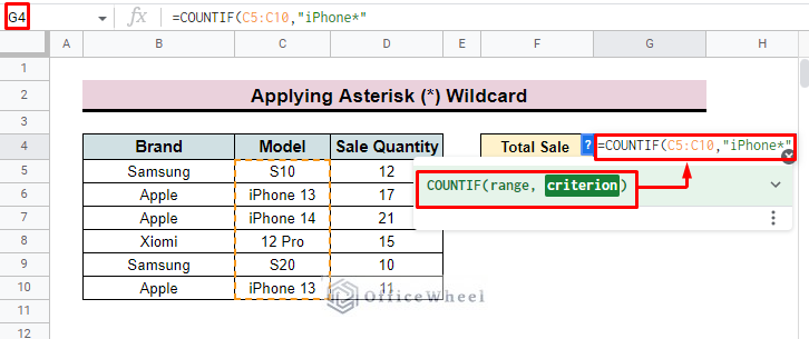
- To apply the function press, ENTER and get the desired result in the selected cell.
=COUNTIF(C5:C10,"iPhone*")Read more: How to Check If Value Exists in Range in Google Sheets (4 Ways)
1.2 Filtering with Conditions
In Google Sheets, by using wildcards we can easily filter any data by applying conditions. To do so,
- In the beginning, select the data range which you want to filter. Here, we select the entire dataset B4:D10.
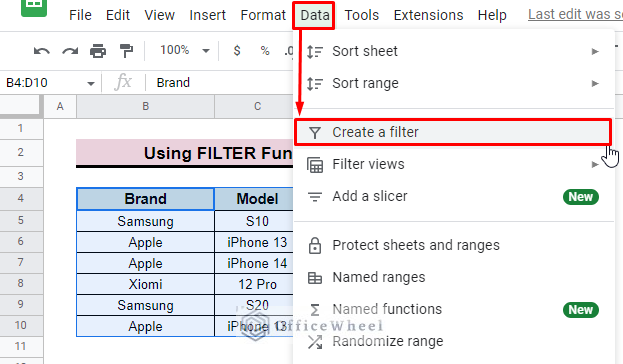
- Then go to the Data bar and select Create a filter option.
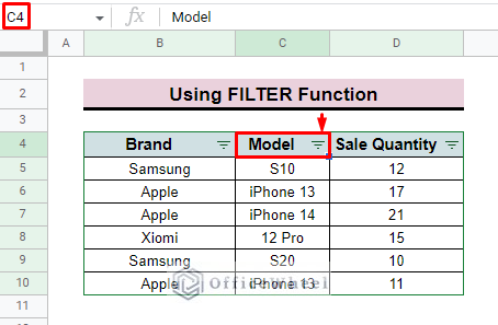
- Yow will find a filter symbol add to every column. Now, go to the column from which basis you want to filter.
- Select Filter by condition.

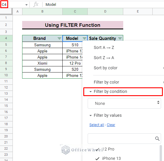
- Then select the Text contains option and insert the value you want to filter. Here, we add iphon*. The * wildcard will help to find this incomplete value easily. In the end, press OK.
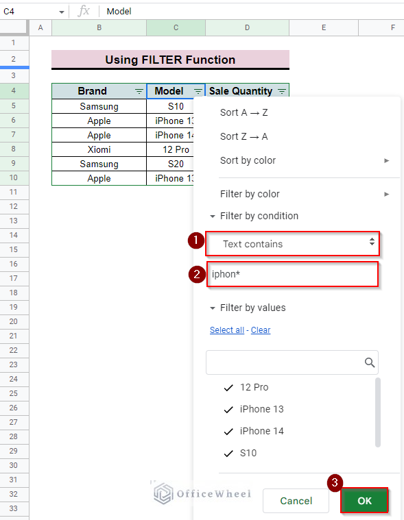
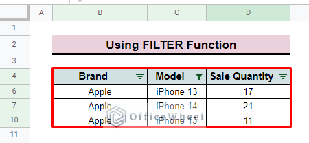
- Finally, you will find all values that contain “iPhone”.
Read More: Google Sheets: Filter Data that Contains Text (3 Easy Ways)
1.3 Performing VLOOKUP with Partial Match
If you want to look up any value that may not exactly match with the source dataset but have a partial match. In that case, the wildcard can be the most useful one. To look up partial value,
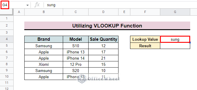
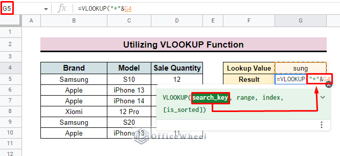
- At the very beginning, insert the partial value in a cell. Here, we look up the partial value “sung” which we insert in cell G4.
- After that in cell G5 apply the VLOOKUP function.
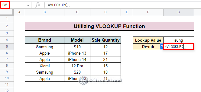
- Add the wildcard with the partial value cell as the search key. Connect the two statements with the “&” symbol. Here, we add the “*” wildcard before the partial value as we look up for the starting value. You can insert it at the end as well as at both sides of the partial value if you look up for the end or middle portion.
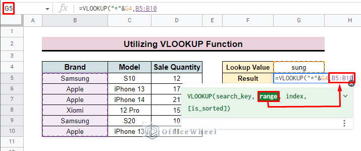
- Then insert the range. Here we add B4:B10.
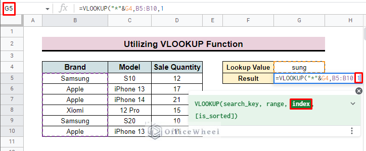
- Add the index which represents the column number. We add 1.
- At the end, set is_sorted FALSE to get the exact result.
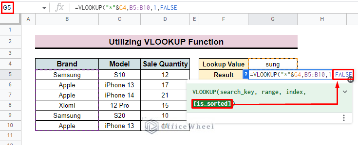
- Finally, press ENTER and you will find the desired result in the selected cell.
=VLOOKUP("*&G4,B4:B10,1,FALSE)Read More: How to VLOOKUP for Partial Match in Google Sheets
Similar Readings
- Set a Filter in Google Sheets (An Easy Guide)
- How to VLOOKUP All Matches in Google Sheets (2 Approaches)
- Delete Filter Views in Google Sheets (An Easy Guide)
- How to Filter Custom Formula in Google Sheets (3 Easy Examples)
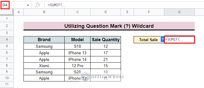
2. Utilizing Question Mark(?) Wildcard
Like the asterisk (*) wildcard the question mark (?) wildcard also helps functions to work more efficiently. As the question mark wildcard represents a single character you have to input the question mark according to the value number. For example, if you want to find two alphabets of any word then you have to put two “?” symbols.
2.1 Applying SUMIF or COUNTIF Functions
In SUMIF and COUNTIF functions, the use of question mark (?) wildcard is the same as the asterisk wildcard.
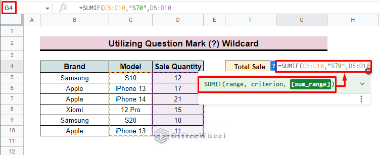
- Input the SUMIF function in cell G4.
- After that enter all the parameters accordingly. For criterion here, we insert “S?0”. So it will sum up all the values that start with S and end with 0.
- Finally, press ENTER and you will find the sum of all S?0 values.
=SUMIF(C5:C10,"S?0",D5:D10)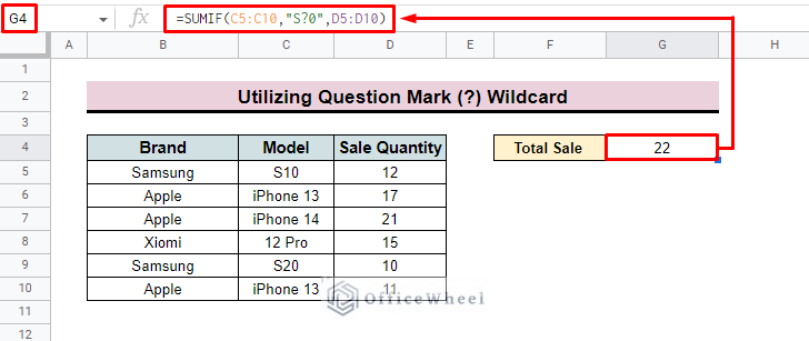
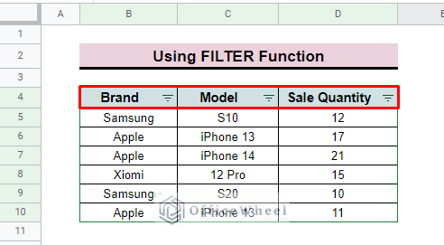
2.2 Conditional Filtering Data
To filter value by using question mark wildcard,
- First, select the entire dataset and insert the filter symbol in all columns by selecting the option Create a filter.
- Then, click on the filter symbol of the column on which basis you filter the entire dataset and go to Filter by conditions>Text contains, insert the value “S?0” and click OK.
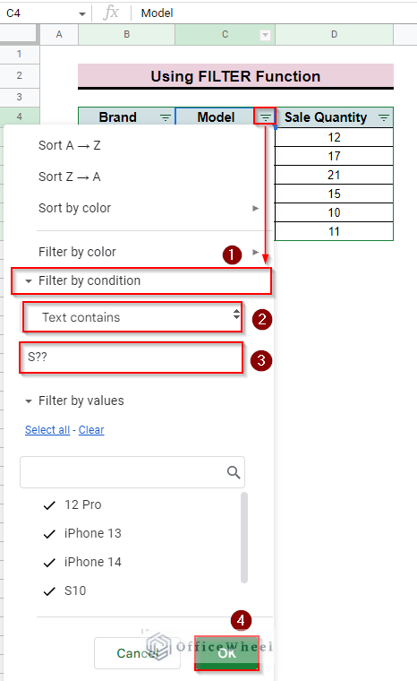
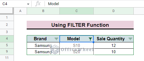
- Finally, you will get the filtered value.
Read More: How to Use Filter with Wildcard in Google Sheets (3 Examples)
2.3 Operating VLOOKUP with Partial Match
As the question mark (?) wildcard represents a single character so you can also look up for partial value by using this wildcard in the VLOOKUP function. To do so,
- First, insert a value you look up for.
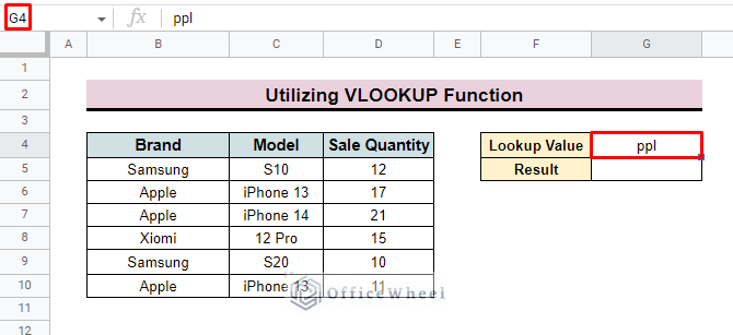
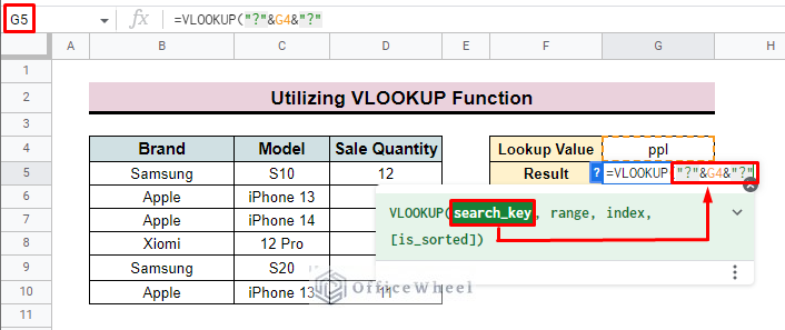
- Then apply the VLOOKUP function in cell G5.
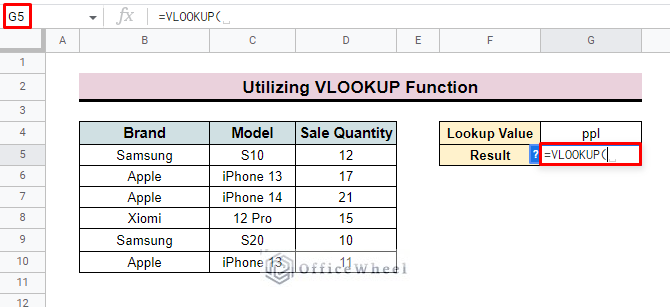
- Now, insert “?”&G4&”?” as the search key. As we have a middle partial value, and we look up the side value that’s why we add the “?” symbol on both sides. Connect all the statements by using the “&” symbol.
- After that, add the range, index, and is_sorted in the same way we applied for the asterisk wildcard at the top.
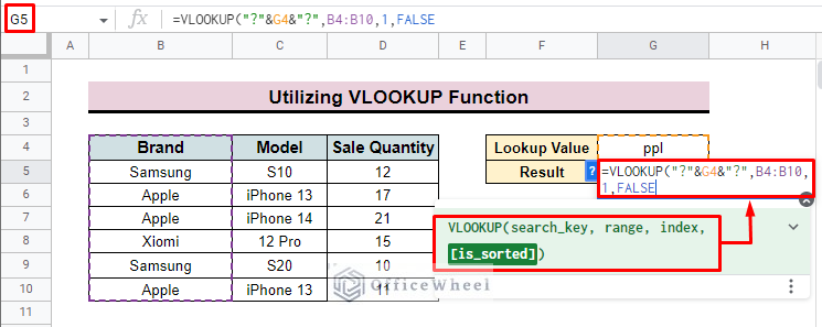
- Finally, press ENTER and you will find the desired look up value in the selected cell.
=VLOOKUP("?&G4&"?",B4:B10,1,FALSE)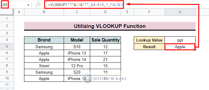
Read More: How to Use VLOOKUP Function with Wildcard in Google Sheets
3. Implementing Tilde (~) Wildcard
The Tilde(~) wildcard is not often used but sometimes it can help you run a function smoothly. It is basically used with other wildcards to indicate that those wildcards are used as simple characters but not wildcards.
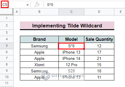
To show the use of a tilde wildcard,
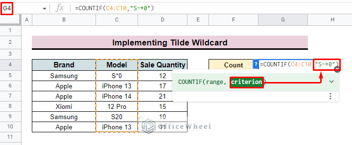
- First, we insert a value S*0 that contains an asterisk wildcard in the dataset.
- Then, apply the COUNTIF formula where the search key is S*0. So, the function counts all partial values including the exact S*0.
=COUNTIF(C4:C10,"S*0")
- We only want to count the S*0 value where the * is not used as a wildcard. So, we insert the Tilde(~) wildcard after the * symbol in the function.
- Finally, press ENTER and you will find that the * symbol counts as a simple character, and the function count only the “S*0” value.
=COUNTIF(C4:C10,"S~*0")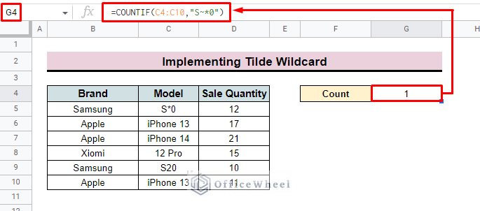
Things to Remember
- In the VLOOKUP function insert the wildcards carefully with partial values.
- The Tilde(~) wildcard always insert after other wildcards.
Conclusion
We hope that you will clearly understand of a wildcard in Google Sheets. To dive deep and explore more about Google Sheets you can visit the OfficeWheel website anytime.
Related Articles
- How to Use Wildcard with IF Condition in Google Sheets (3 Ways)
- [Fixed!] Wildcard Is Not Working in Google Sheets (5 Solutions)
- How to Use QUERY Function with Wildcard in Google Sheets
- Filter Based on a Cell Value in Google Sheets (2 Easy ways)
- Find and Replace with Wildcard in Google Sheets
- Google Sheets: The FILTER Function (A Comprehensive Guide)
- Filter by Condition Using a Custom Formula in Google Sheets (3 Easy Examples)