The VLOOKUP function is a vast tool in Google Sheets. You can perform numerous types of calculations using this function in Google Sheets. In this article, I’ll show 4 useful examples to Concatenate with VLOOKUP in Google Sheets with clear images and steps.
A Sample of Practice Spreadsheet
You can download Google Sheets from here and practice very quickly.
4 Suitable Examples to Concatenate with VLOOKUP in Google Sheets
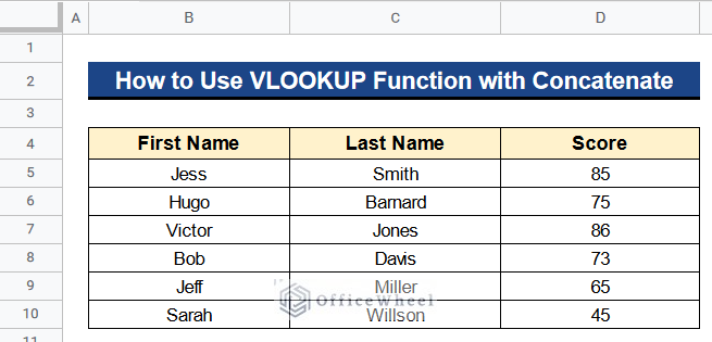
Let’s get introduced to our dataset first. Here we have the first names of some people in Column B, their last names in Column C and their scores in Column D. Now I’ll show you 4 suitable examples to Concatenate with VLOOKUP in Google Sheets with the help of this dataset.
Example 1: Using VLOOKUP and CONCATENATE Functions
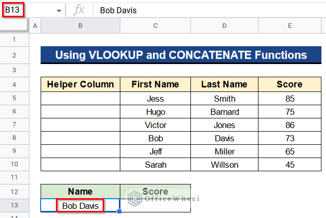
Now we have a full name in Cell B13 of our dataset as you can see in the picture. Moreover, we want to get his score. But the dataset has separate names in separate columns like Columns C and D. So we’ll use the VLOOKUP and CONCATENATE functions to get unique values in Google Sheets. For this, we’ll first create a helper column in Column B. Then, the CONCATENATE function will connect the values together. And the VLOOKUP function will search for the unique values.
Steps:
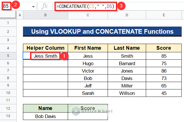
- Firstly, type the following formula in Cell B5–
=CONCATENATE(C5," ",D5)- Secondly, hit Enter to get the names together.
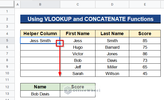
- Next, you’ll get all the names concatenated in Column B.
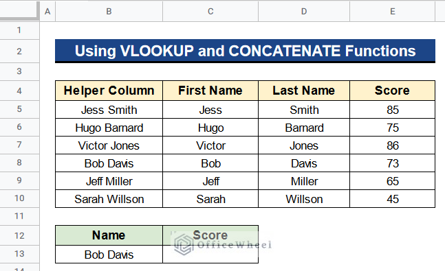
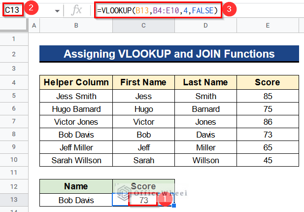
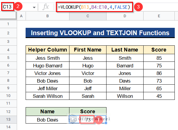
- Then, write the following formula in Cell C13–
=VLOOKUP(B13,B4:E10,4,FALSE)- After that, press Enter to get the score.
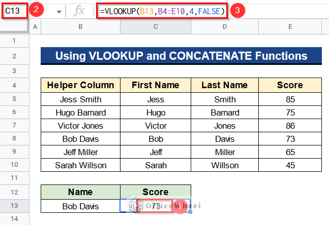
- Finally, we are getting results for unique values using the VLOOKUP and CONCATENATE functions in Google Sheets.
Read More: How to Concatenate with VLOOKUP in Google Sheets
Example 2: Applying Concatenate Operator and VLOOKUP Function
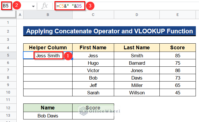
Unlike, the previous method we can use the Concatenate Operator (&) and the VLOOKUP function to concatenate two columns in Google Sheets. The Concatenate Operator (&) will connect the two columns, Columns C and D. After that, the VLOOKUP function will look for the given value which is the full name.
Steps:
- First of all, insert the following formula in Cell B5–
=C5&" "&D5- Afterward, click Enter to get the result.
- Again, use the Fill Handle tool for the rest of the cells of Column B.
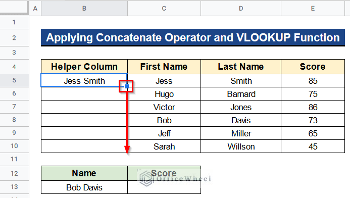
- At last, you’ll see that values from Columns C and D are concatenated in Column B.
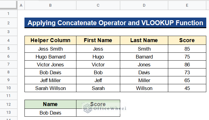
- Then, put the following formula in Cell C13–
=VLOOKUP(B13,B4:E10,4,FALSE)- Finally, hit the Enter Button to get the score.
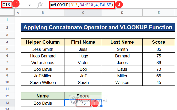
- Ultimately, we have applied the Concatenate Operator (&) and the VLOOKUP function to concatenate two columns, Columns C and D, and get results from them.
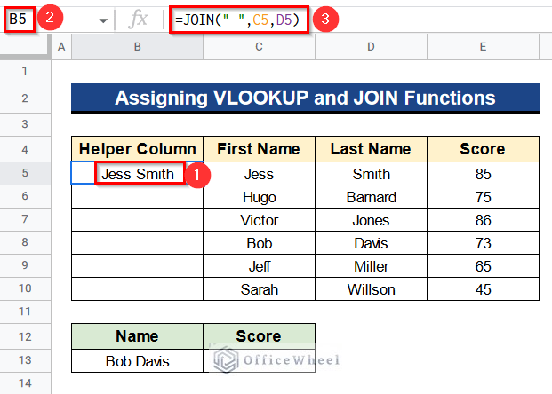
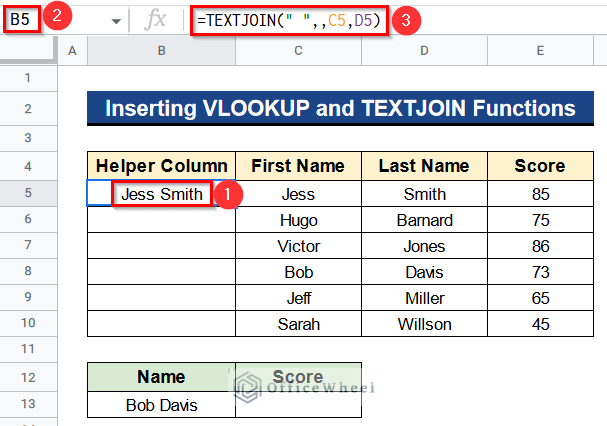
Example 3: Assigning VLOOKUP and JOIN Functions
Similarly, we can assign the VLOOKUP and JOIN functions to concatenate multiple values in Google Sheets. The JOIN function will connect the values together from Columns C and D. Then, the VLOOKUP function will search for the unique value which is the full name in the dataset.
Steps:
- In the first place, type the following formula in Cell B5–
=JOIN(" ",C5,D5)- Consequently, press the Enter Button to get the output.
- Next, assign the Fill Handle tool to get the names in the rest of the cells of Column B.
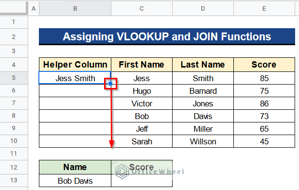
- After that, you’ll find that multiple values concatenated in the helper column, Column B.
- Thereafter, write the following formula in Cell C13–
=VLOOKUP(B13,B4:E10,4,FALSE)- Afterward, click the Enter Button to get the score related to the name.
- In the end, we are getting output for multiple values.
Read More: How to Use the VLOOKUP Function in Google Sheets
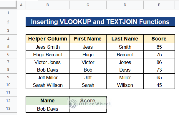
Example 4: Inserting VLOOKUP and TEXTJOIN Functions
Apart from the previous methods, we can also insert the VLOOKUP and TEXTJOIN functions to concatenate multiple columns or values in Google Sheets. In this process, the TEXTJOIN function will join the two names from Columns C and D. Then the VLOOKUP function will look for their scores in Column E.
Steps:
- In the beginning, insert the following formula in Cell B5–
=TEXTJOIN(" ",,C5,D5)- Consequently, hit Enter to get the names together.
- Again, use the Fill Handle tool for Column B to get the remaining output.
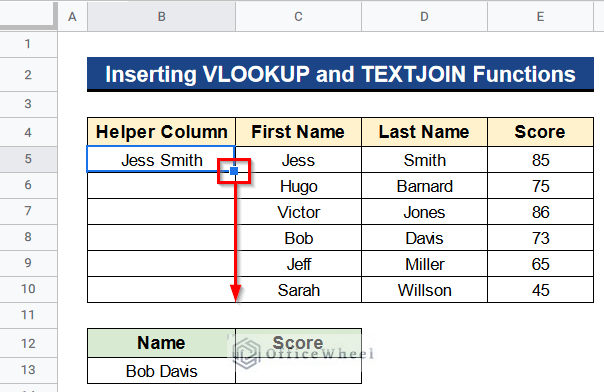
- Moreover, the concatenated values will be in Column B.
- Then, put the following formula in Cell C13–
=VLOOKUP(B13,B4:E10,4,FALSE)- Next, press Enter to get the desired score.
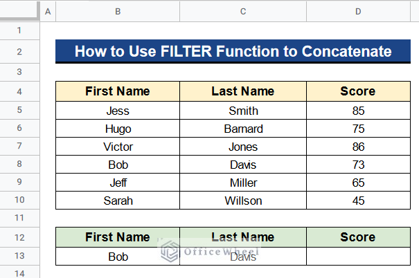
How to Use FILTER Function to Concatenate in Google Sheets Instead of VLOOKUP Function
We have a different situation now. The first name and last name lie separately in our dataset below under Column B and Column C. Now, I want to look for the score from Column D based on these two separate values. At this moment we can use the FILTER function alone to Concatenate in Google Sheets instead of the VLOOKUP function. The FILTER function will search for these two values together in our dataset and give the result instantly. Let’s see the steps.
Steps:
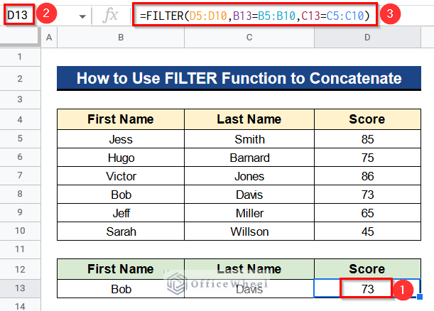
- Before all, write the following formula in Cell D13–
=FILTER(D5:D10,B13=B5:B10,C13=C5:C10)- Finally, click Enter to get the score quickly.
Read More: How to VLOOKUP with Multiple Criteria in Google Sheets
Conclusion
That’s all for now. Thank you for reading this article. In this article, I have discussed 4 suitable examples to Concatenate with VLOOKUP in Google Sheets. I have also discussed using the FILTER function alone to Concatenate in Google Sheets instead of the VLOOKUP function. Please comment in the comment section if you have any queries about this article. You will also find different articles related to google sheets on our officewheel.com. Visit the site and explore more.