We use the VLOOKUP function often to lookup for values in our dataset. However, sometimes Google Sheets users get different errors while applying the function. Though these errors mostly happen due to minor mistakes and are very easy to resolve quickly. In this article, we will discuss the VLOOKUP error and how to avoid these errors in Google Sheets. Read along to know more on this topic.
A Sample of Practice Spreadsheet
You can download the practice spreadsheet from the download button below.
5 Most Frequent VLOOKUP Errors in Google Sheets
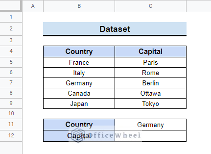
Suppose, you have a dataset that contains the names of some countries and their capital city names. You will use the VLOOKUP function to find the capital name in the blank search box.
Now, you can get various errors while using the VLOOKUP function in this dataset. We will show you the errors that can happen while using the function and the steps on how to solve them. So, read along to know the VLOOKUP error in Google Sheets.
1. VLOOKUP #N/A Error
One common error while using the VLOOKUP function is the #N/A Error. This means “ No value is available”. This is a simple error and it can be resolved by taking an easy step.
- First, select cell C12 and insert the below formula in the formula bar.
=VLOOKUP(C11,B5:C9,2,0)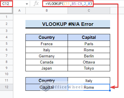
- Now, the syntax of the VLOOKUP function is:
VLOOKUP(search_key, range, index, [is_sorted])
The search key should be included in the table. If you insert any data/value that is not already in the table, then it will show a #N/A Error.

Solution:
You can insert the proper search key from the data table to avoid this Error. You can also use the IFNA function with the VLOOKUP function to avoid seeing the error.
- First, insert the below formula instead of the previous formula.
=IFNA(VLOOKUP(C11,B5:C9,2,0))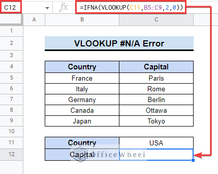
- This formula will replace the error with a blank.
- If you want to show any text or number in the blank, you can type like the below-mentioned formula.
=IFNA(VLOOKUP(C11,B5:C9,2,0),"No Data")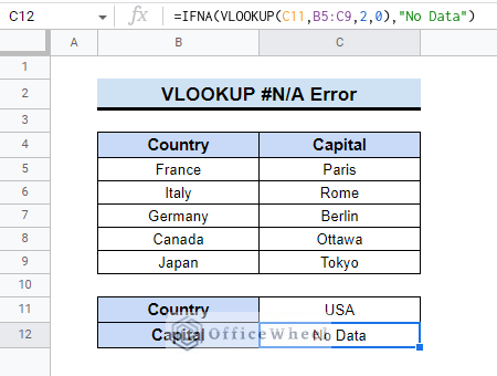
Read More: Alternative to Use VLOOKUP Function in Google Sheets
2. #REF! Error
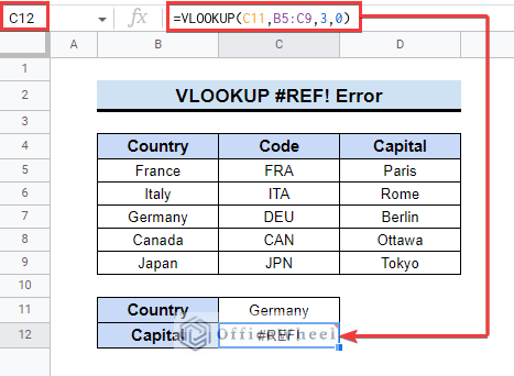
Another common error in applying the VLOOKUP function in Google Sheets is #REF! Error. It happens when you don’t apply the correct reference range in the formula. Follow the steps to know the error and its solution.
- First, apply the below formula in cell C12.
=VLOOKUP(C11,B5:C9,3,0)- After that, you will see #REF! Error in cell C12 because here in the formula, you are looking for the capital city name of a country, which is in the D column, but your reference range has no D column in it. This is why the error is showing.
Solution:
- Now, if you want to solve this error then put the below formula in the cell.
=VLOOKUP(C11,B5:D9,3,0)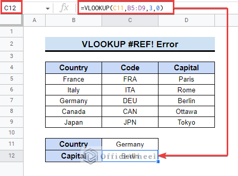
- At this time, you can see the formula range is B5:D9. So, it contains the proper reference range. That is why there is no #REF!
Similar Readings
- VLOOKUP with IMPORTRANGE Function in Google Sheets
- Highlight Cell If Value Exists in Another Column in Google Sheets
- How to Use VLOOKUP for Conditional Formatting in Google Sheets
- Concatenate with VLOOKUP in Google Sheets
- How to Use VLOOKUP with IF Statement in Google Sheets
3. #VALUE! Error
You can also get #VALUE! Error while utilizing the VLOOKUP function in Google Sheets. This happens when you put the arguments in the wrong order.
- First, insert the following formula in cell C12.
=VLOOKUP(B5:C9,C11,2,0)
- And, you will get a #VALUE! Error for the wrong use of syntax. Here, in this formula, the range is in the first place and then the search key, which is in the wrong order. This is the reason for the error.
Solution:
Just write the formula following the correct syntax then you will not get this kind of error.
=VLOOKUP(C11,B5:C9,2,0)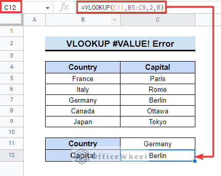
Read More: How to Check If Value Exists in Range in Google Sheets (4 Ways)
4. VLOOKUP #NAME? Error
If you make a mistake while typing the function name then you will get a #NAME? Error. Follow the steps below to see the error and know how to avoid or resolve it.
- First, enter the following formula in a cell.
=VLOOKU(C11,B5:C9,2,0)- As you can see, there is a typo in the function name. This is why the output is showing a #NAME?
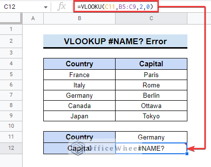
Solution:
- If you put the function name correctly like the below-mentioned formula then this error will not occur.
=VLOOKUP(C11,B5:C9,2,0)
5. #ERROR! Error
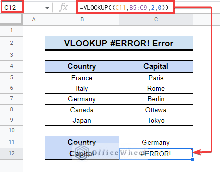
There is another type of error that occurs during using the VLOOKUP function, that is #ERROR! Error. When there is a parenthesis error in the formula, then this error is displayed. Read the following steps to know the error and its solution.
- First, insert the following formula selected cell.
=VLOOKUP((C11,B5:C9,2,0))- Then, you will see the #ERROR! error in return.
- Now, if you check properly, you will see there are double parentheses in the formula. This is the reason for the error.
Solution:
Put parenthesis properly in the formula like below to avoid parse errors.
=VLOOKUP(C11,B5:C9,2,0)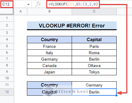
Things to Remember
- Please keep in mind, the index of the VLOOKUP function should never be 0. As it means the number of a column so it should be any number other than zero.
- In the VLOOKUP function, the lookup value must be in the leftmost or first column in the given reference range.
Conclusion
We have tried to show you the VLOOKUP error in Google Sheets. Hopefully, the examples above will be enough for you to understand the errors of the function and their solutions. You can practice using the sample spreadsheet. Please use the comment section below for further queries or suggestions. You may also visit our OfficeWheel blog to explore more about Google Sheets.
Related Articles
- Google Sheets Vlookup Dynamic Range
- How to Use VLOOKUP with Named Range in Google Sheets
- Use Wildcard in Google Sheets (3 Practical Examples)
- How to Use Nested VLOOKUP in Google Sheets
- [Fixed!] Google Sheets If VLOOKUP Not Found (3 Suitable Solutions)
- How to VLOOKUP for Partial Match in Google Sheets
- VLOOKUP Multiple Columns in Google Sheets (3 Ways)
- How to Use VLOOKUP to Import from Another Workbook in Google Sheets