How to Highlight Row If Cell Is Not Empty in Google Sheets

We can always highlight any row or column manually in Google Sheets. But the automatic process of highlighting row if a cell is not empty in Google Sheets is ordinary and straightforward. We can use the Conditional formatting feature for this purpose. In this article, you’ll find several processes to highlight row if cell is not empty in Google Sheets.

A Sample of Practice Spreadsheet

You can download Google Sheets from here and practice very quickly.

7 Simple Methods to Highlight Row If Cell Is Not Empty in Google Sheets

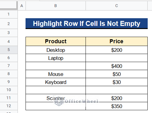
At first, let’s get introduced to our dataset. Here we have products in Column B and their price in Column C. You may notice some of the values are missing here. These cells are empty. We have to highlight row if cell is not empty in Google Sheets. We can do this conveniently by using Conditional formatting. Now I’ll show you 7 methods of Conditional formatting to highlight row if cell is not empty in Google Sheets.

1. Applying Cell Is Not Empty Command

There is a direct command in Google Sheets for quickly highlighting the non-blank cells. The command is called Cell is not empty command.

Steps:

• Firstly go to Format > Conditional formatting.

• Secondly, give the data range from Cell B5 to C12.
• Then select Is not empty under the Format rules menu.
• After that, select green color from the Color Button.
• Finally, click the Done Button.

• At last, you’ll get the rows highlighted if the cell contains text as shown in the image.

Read More: Google Sheets: Highlight Row If Cell Is Empty

2. Using Custom Formula Command

We can also highlight rows if the cell contains a text by using the Custom formula Command under the Conditional formatting menu. You’ll get the output by just typing the formula swiftly.

Steps:

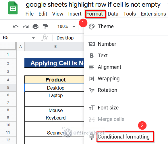
• First, go to Format > Conditional formatting as shown in the first step of Method 1.
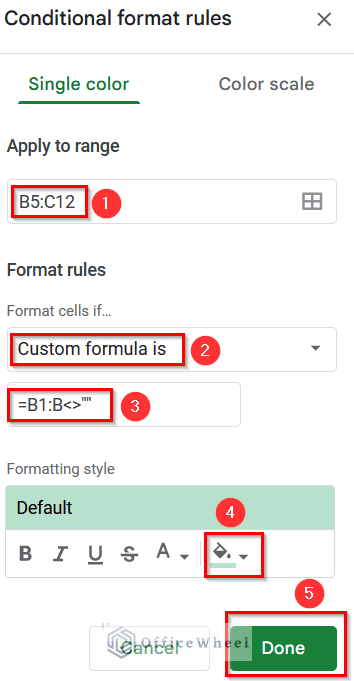
• Second, give the data range from Cell B5 to C12.
• After that, select Custom formula is under the Format rules menu and type the following formula-

• Then select the green color from the Fill Color Button.
• At last, click the Done Button.

• Finally, you’ll get the highlighted rows that have values.

Read More: Conditional Formatting with Multiple Conditions Using Custom Formulas in Google Sheets

3. Inserting NOT Function

Moreover, we can use the NOT function. When we put this function in the Conditional formatting menu the result is automatic.

Steps:

• Foremost, go to Format > Conditional formatting like the first step of Method 1.
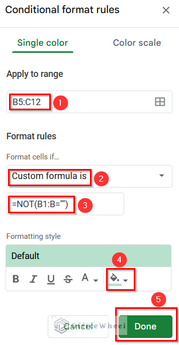
• Thereafter, give the data range from Cell B5 to C12.
• Later, select Custom formula is under the Format rules menu and write the following formula-

• Consequently, select green color from the Fill Color Button.
• Eventually, click the Done Button.

• Ultimately, you’ll get the output.

Read More: How to Use VLOOKUP for Conditional Formatting in Google Sheets

4. Using IF Function

Additionally, we may use the IF function to get the highlighted rows if the corresponding cells contain any value. The process is straightforward.

Steps:

• In the beginning, go to Format > Conditional formatting kind of the first step of Method 1.
• Next, give the data range from Cell B5 to C12.
• Then, select Custom formula is under the Format rules menu and inscribe the following formula-

• Hereafter, select green color from the Color Button.
• Finally, click the Done Button.

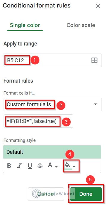
• In the end, you’ll get the desired result.

Read More: How to Use IF Function in Google Sheets (6 Suitable Examples)

Similar Readings

• How to Use Multiple IF Statements in Google Sheets (5 Examples)
• Highlight Row Based on Date in Google Sheets (2 Suitable Ways)
• How to Use AND Function in Google Sheets (4 Useful Examples)
• Use ARRAYFORMULA with IF Function in Google Sheets
• Find if Date is Between Dates in Google Sheets (An Easy Guide)

5. Combining NOT and ISBLANK Functions

Further, we can use the combination of NOT and ISBLANK functions to get our desired result. We have to just write the formula properly in the Conditional formatting menu.

Steps:

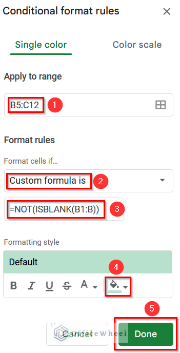
• Before all, go to Format > Conditional formatting as in the first step of Method 1.
• Secondly, give the data range from Cell B5 to C12.
• Later, select Custom formula is under the Format rules menu and type the following formula-

• Then, select green color from the Fill Color Button.
• Lastly, click the Done Button.

• Finally, you’ll get the rows highlighted as shown in the image.

Read More: How to Highlight Active Row in Google Sheets (2 Suitable Ways)

6. Inserting LEN Function

Now, look into a different condition. We want to highlight those rows which have values in Column B. We don’t care about the values of Column C. But we want to highlight both columns based on the values of Column B. So we can satisfy the condition by using the LEN function.

Steps:

• In the beginning, go to Format > Conditional formatting like the first step of Method 1.
• Then, give the data range from Cell B5 to C12.
• After that, select Custom formula is under the Format rules menu and write the following formula-

• Then, select green color from the Fill Color Button.
• At last, click the Done Button.

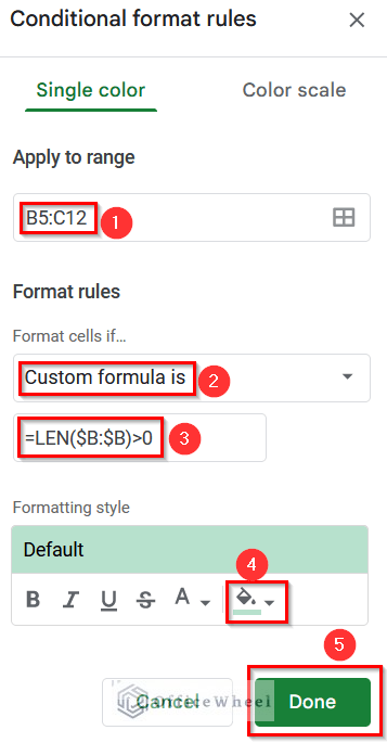
• Ultimately, you’ll find that only those rows are highlighted which have values in Column B. As an example, Cell B7 doesn’t have any value but Cell C7 has a value. So Row 7 isn’t highlighted.

Read More: How to Highlight Every Other Row in Google Sheets (2 Methods)

7. Merging AND, NOT, and ISBLANK Functions

Again we have a different condition. Now we want to only highlight the cells of Column B which have values in them. But we also want to add a condition that Column C should also have a value in order to highlight cells of Column B. These can be done by merging the AND, NOT, and ISBLANK functions together. The output is fast.

Steps:

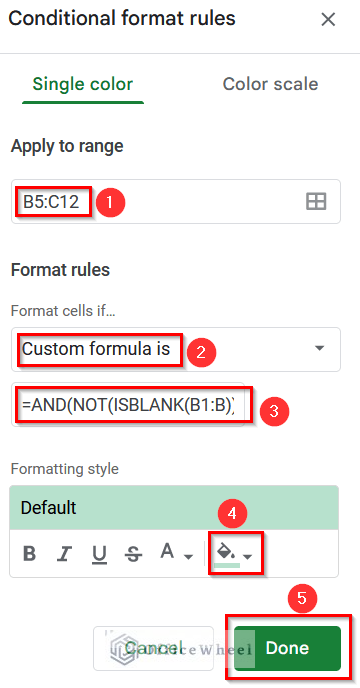
• Firstly, go to Format > Conditional formatting as shown in the first step of Method 1.
• Secondly, give data range from Cell B5 to C12.
• Then, select Custom formula is under the Format rules menu and insert the following formula-

• Next, select green color from the Color Button.
• Last but not the least, click the Done Button.

• In the final phase, you’ll see that only those cells of Column B are highlighted that have values with respect to the values of Column C. Like, Cell B6 doesn’t get highlighted because its corresponding cell, Cell C6 is empty.

Read More: Google Sheets: Conditional Formatting with Multiple Conditions

Conclusion

That’s all for now. Thank you for reading this article. In this article, I have tried to discuss 7 different methods of conditional formatting to highlight row if cell is not empty in Google Sheets. Please comment in the comment section if you have any queries about this article. You will also find different articles related to google sheets on our officewheel.com. Visit the site and explore more.

Related Articles

• How to Highlight Highest Value in Row in Google Sheets (2 Ways)
• Use REGEXMATCH Function for Multiple Criteria in Google Sheets
• How to Highlight a Row If Date in Cell Is Today in Google Sheets
• Use Nested IF Function in Google Sheets (4 Helpful Ways)
• Filter Values that Contains Multiple Text Criteria in Google Sheets (2 Easy Ways)
• How to Use IF and OR Formula in Google Sheets (2 Examples)
• Use IF Condition Between Two Numbers in Google Sheets