Highlighting a row based on today’s date is quite easy to achieve if you know the right method. In this article, we will discuss how to highlight a row if the date in the cell is today in Google Sheets using a custom formula.
A Sample of Practice Spreadsheet
3 Examples to Highlight a Row If Date in Cell Is Today in Google Sheets
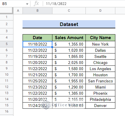
To begin the process, we need to have a dataset with Dates on it. The date format we will be using is MM/DD/YYYY. You can use any other format you like. We have a dataset with the Date, Sales Amount, and City Name for the month of November 2022. This dataset will be used by us to highlight rows based on today’s date.
1. Entire Row Highlighting
We need to use a custom formula in conditional formatting to see if any cell contains today’s date and highlight the entire row easily. Follow these steps:
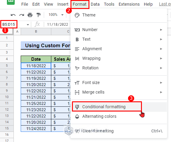
- First, select the range of tables where you want the highlight to take place. We select the range B5:D15.
- Then, go to Menu bar > Format > Conditional formatting.
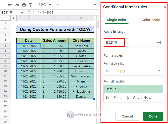
- Now, you will see a sidebar called Conditional format rules appear on the right. The sidebar specifies where it is applying the formatting in the Apply to range In our example, it says B5:D15.
- Next, from the Format rules tab from the Format cells if drop-down menu, select the Custom formula is option.
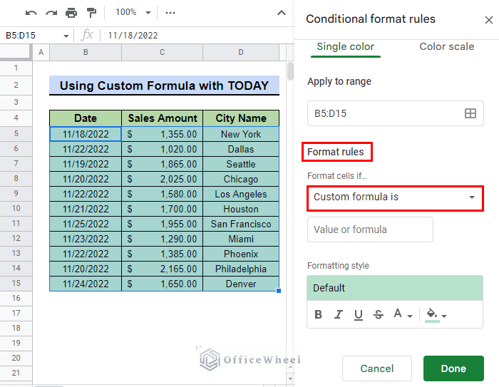
- Then, in the Value or formula box type in the following custom formula:
=$B5=TODAY()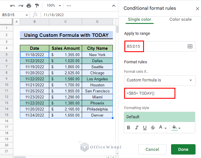
Formula Explanation:
- B5 denotes the first cell in the range where the date is located. We used absolute cell references ($) to lock the column. Conditional formatting will match this value.
- TODAY() specifies if it is indeed today’s date or not.
- If conditional formatting finds an exact match then it will highlight the entire row.
- You can format the table further in the Formatting style You can select a custom font size and a preferred color. We select light red 2 for our example.
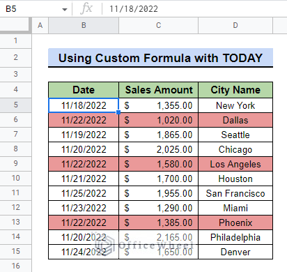
- Finally, press Done and your rows are now highlighted based on today’s date.

- This is what the final table looks like:
Read More: Highlight Row If Cell Contains Text with Conditional Formatting in Google Sheets
Similar Readings
- How to Highlight Every Other Row in Google Sheets (2 Methods)
- Highlight Lowest Value in Row in Google Sheets (2 Easy Ways)
2. Before or After Today’s Date
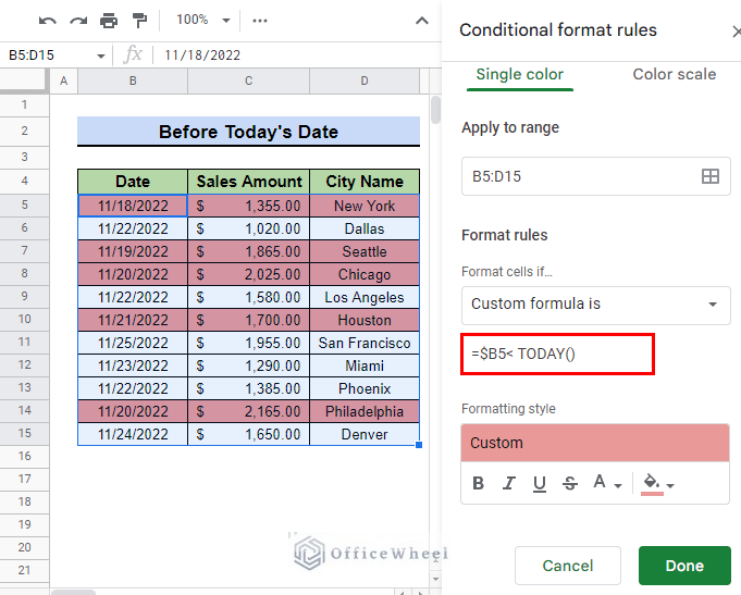
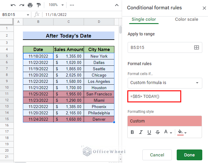
You can also highlight rows if the dates are before or after today’s date by simply replacing = with < or > operators in the formula or typing in the following formulas:
=$B5<TODAY()Less-than sign (<) will find the dates that are before today’s date and highlight the rows based on that. Since dates before have a lower numerical value.
=$B5>TODAY()Greater-than sign (>) will find the dates that are after today’s date and highlight the rows based on that. Since dates after have a higher numerical value.
Read More: Highlight Row Based on Date in Google Sheets (2 Suitable Ways)
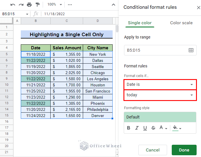
3. Highlighting Only a Single Cell
You can highlight only the cells containing today’s dates using the default conditional formatting option in Google Sheets. Follow these steps:
- First, open the conditional formatting side panel.
- Next, from there select the Date is option from Format cells if drop-down under the Format rules tab
- Then, select today.
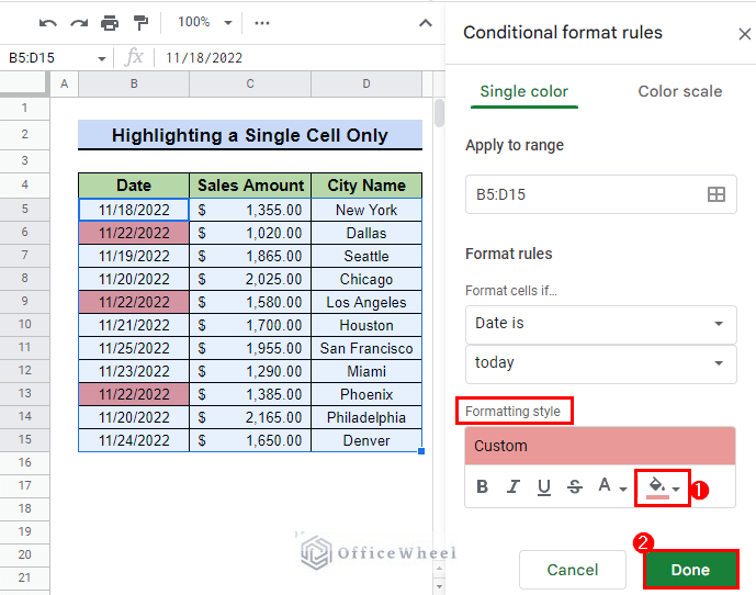
- You can customize your highlighted column from the Formatting style menu if you don’t like the default style. We went with light red 2 as a formatting style for our example.
- Finally, press Done and you can now see the cells are highlighted according to today’s date.
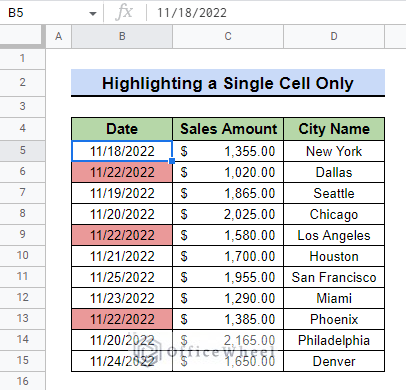
- This is what the table looks like:
Read More: How to Highlight Row If Cell Is Not Empty in Google Sheets
Conclusion
In this article, we showed you how to highlight a row based on today’s date in Google Sheets with a custom formula. We hope this article was useful to you. Keep practicing the method we have shown here to better understand the concept.
Also, check out other articles on OfficeWheel to keep on improving your Google Sheets work knowledge.