If you need to highlight row based on a date in Google Sheets then you have come just to the right place! In this article, we will discuss in detail how you can highlight row based on a date in Google Sheets and can apply the learning in your daily life easily and effectively. We will use conditional formatting to highlight rows in this article.
A Sample of Practice Spreadsheet
2 Methods to Highlight Row Based on Date in Google Sheets
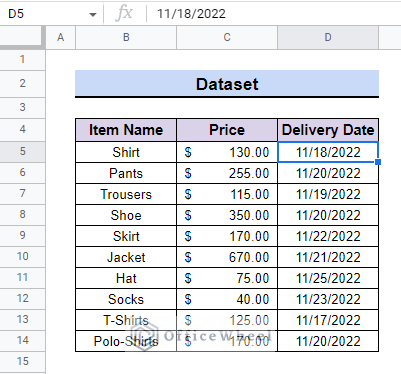
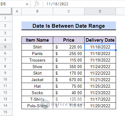
To begin the process, we need to have a dataset with Dates on it. The date format we will be using is: MM/DD/YYYY. You can use any other format you like. We have a dataset with Item Name, Price, and Delivery Date. We will use this dataset to highlight row based on date.
1. Based on Today’s Date
We can use a custom formula in Conditional formatting to see if any cell contains today’s date and highlight the entire row easily.
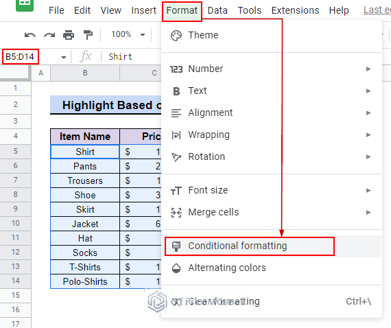
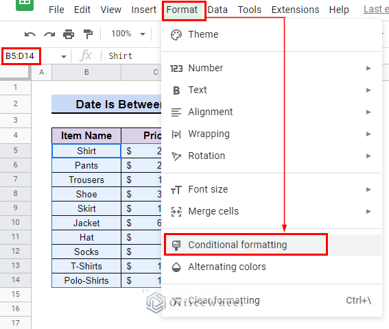
- First, select the range of tables where you want the highlight to take place. We select the range B5:D14.
- Then, go to Menu bar > Format > Conditional formatting.
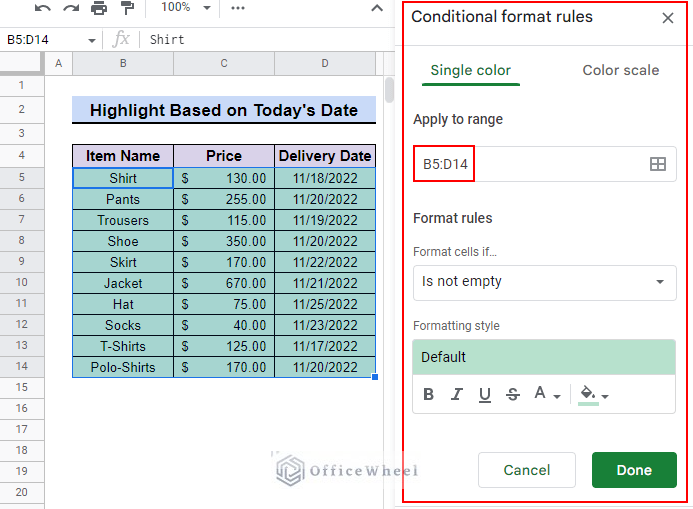
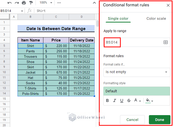
- Now, you will see a sidebar appear from the right-hand side. The sidebar specifies where it is applying the Conditional formatting in the Apply to range In our example, it says B5:D14.
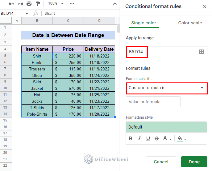
- Next, from the Format rules tab from Format cells if box select Custom formula is option.
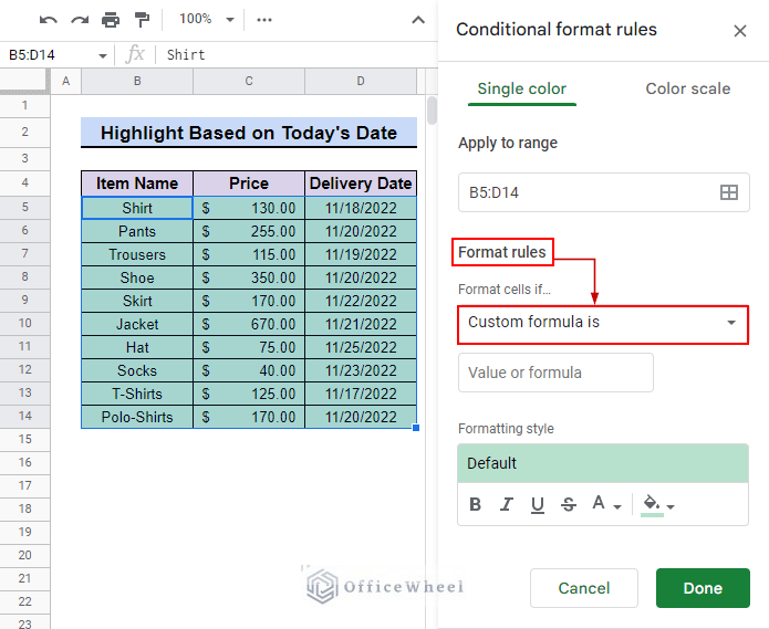
- Then, in the Value or formula box type in the following formula:
=$D$5:$D$14 = TODAY()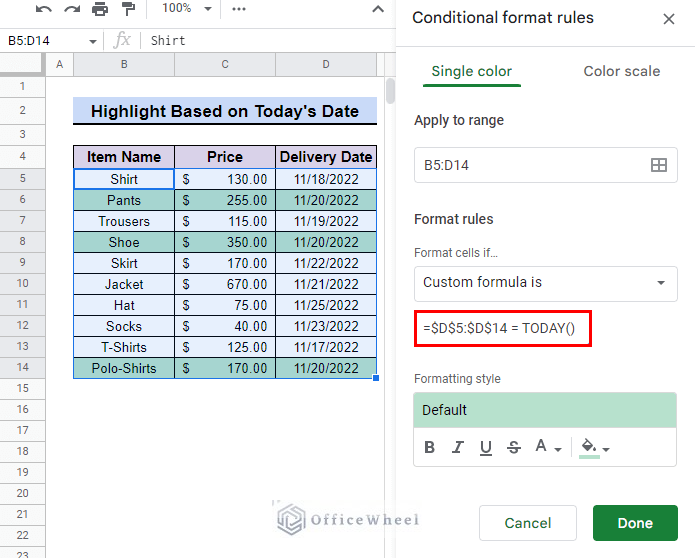
Formula Explanation:
- D5:D14 denotes the column of date. We used absolute cell references ($) to lock the column.
TODAY()specifies if it is indeed today’s date or not.
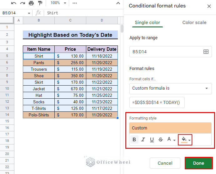
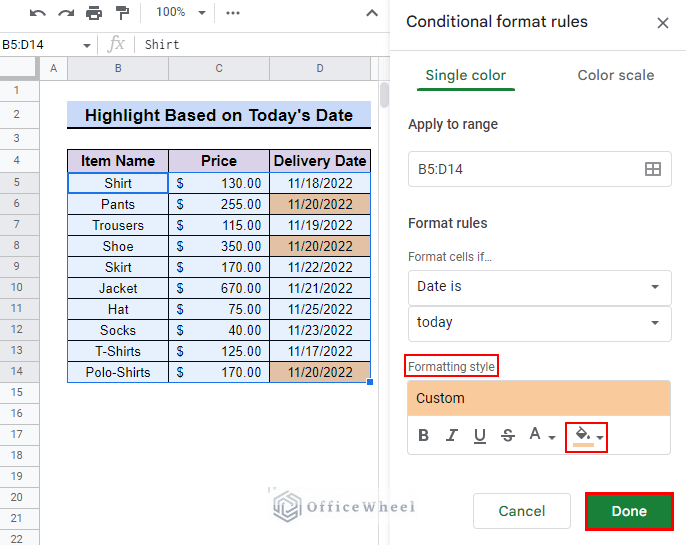
- You can format the highlighted table further in the Formatting style You can select a custom font size and even select a preferred color. We select light orange 2 for our example.
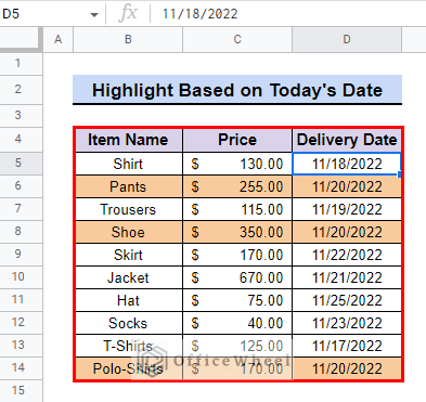
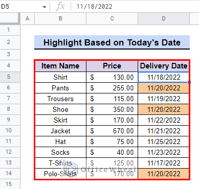
- Finally, press Done your rows are now highlighted based on today’s date.
- This is what the final table looks like:
You can also highlight dates if the dates are before or today’s date by simply replacing = with < or > in the formula or typing in the following formulas:
For dates before today:
=$D$5:$D$14 < TODAY()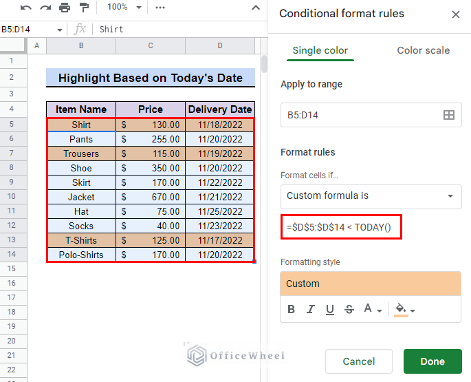
For dates after today:
=$D$5:$D$14 > TODAY()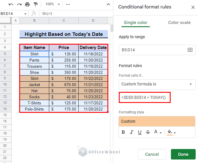
Read More: How to Highlight Row If Cell Is Not Empty in Google Sheets
Highlight Single Cell Based on Today’s Date
You can highlight only the cells of today’s dates using the default method in Google Sheets.
- First, go to Menu bar > Format > Conditional formatting.
- Now, you will see a sidebar appear from the right-hand side. The sidebar specifies where it is applying the Conditional formatting in the Apply to range In our example, it says B5:D14.
- Next, from the Format rules tab from Format cells if box select Date is option.
- Then, select today.
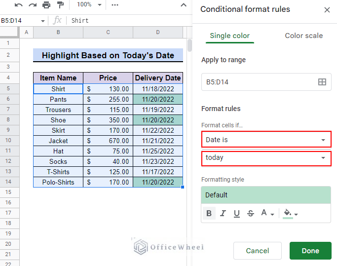
- You can format the highlighted table further in the Formatting style You can select a custom font size and a preferred color. We selected light orange 2 for our example.
- Finally, press Done and you can now see the cells are highlighted according to today’s date.
This is what the table looks like:
Read More: How to Highlight a Row If Date in Cell Is Today in Google Sheets
2. If the Date Is Between a Range of Dates
You can use a custom formula with Conditional formatting to highlight the entire row if a date is between a range of dates in Google Sheets. We need to introduce AND and DATE functions if we want to highlight rows with a date between a range of dates.
For this, we can use the same dataset used in the previous method.
Follow these steps:
- First, select the range of tables where you want the highlight to take place. We select the range B5:D14.
- Then, go to Menu bar > Format > Conditional formatting.
- Now, you will see a sidebar appear from the right-hand side. The sidebar specifies where it is applying the Conditional formatting in the Apply to range In our example, it says B5:D14.
- Next, from the Format rules tab from Format cells if box select Custom formula is option.
- Then, type in the following formula:
=AND($D5<=DATE(2022,11,21),$D5>=DATE(2022,11,19))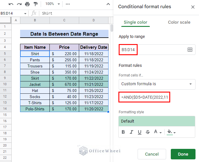
Formula Explanation:
- D5 denotes the column where the date is located. Notice how we partially locked D5.
- 2022,11,21(YYYY,MM,DD) and 2022,11,19(YYYY,MM,DD) denote the range of dates. If the said date is between this date range then the entire row will be highlighted.
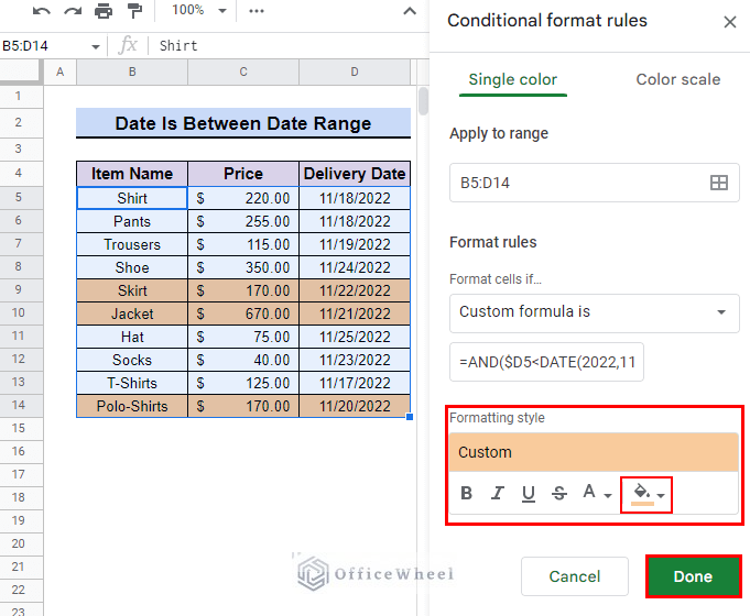
- Then, you can format the highlighted table further in the Formatting style. From there you can select a custom font size and a preferred color too. You can even select custom formatting options. We select light orange 2 for our example.
- Finally, press Done and your rows are now highlighted based on today’s date.
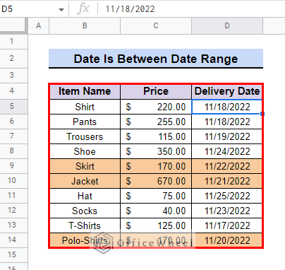
- This is what the final table looks like:
Read More: Conditional Formatting with Multiple Conditions Using Custom Formulas in Google Sheets
Similar Readings
- How to Use VLOOKUP for Conditional Formatting in Google Sheets
- Google Sheets: Highlight Row If Cell Is Empty
- How to Highlight Active Row in Google Sheets (2 Suitable Ways)
- Google Sheets: Conditional Formatting with Multiple Conditions
- How to Highlight Every Other Row in Google Sheets (2 Methods)
Highlight Single Cell If Date Is Between a Range of Dates
You can highlight only the cells of dates between a date range using the default method in Google Sheets.
- First, go to Menu bar > Format > Conditional formatting.
- Now, you will see a sidebar appear from the right-hand side. The sidebar specifies where it is applying the Conditional formatting in the Apply to range In our example, it says B5:D14.
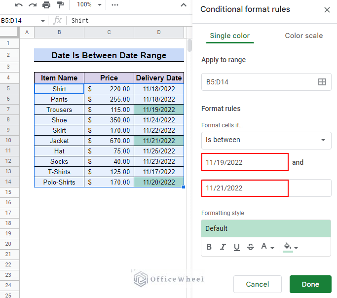
- Next, from the Format rules tab from Format cells if box select is between option.
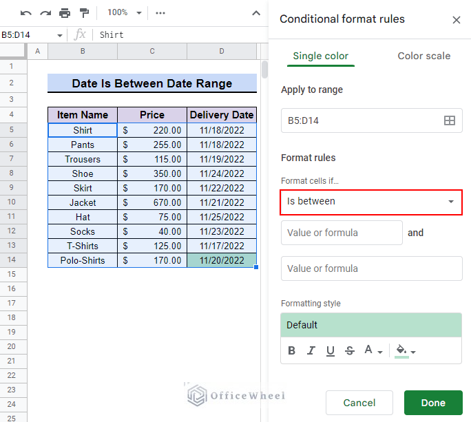
- Then, in the first blank box type in the start range, and in the second blank box type the end range. We type 11/19/2022 and 11/21/2022 respectively.
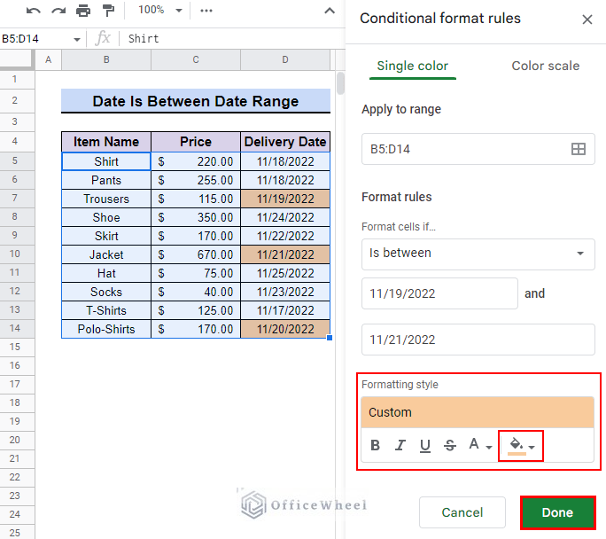
- Now, you can format the highlighted table further in the Formatting style bar. You can select a custom font size and even select a preferred color too according to your choice. We chose light orange 2 for our example.
- Finally, press Done and you can now see the cells are highlighted according to the range specified.
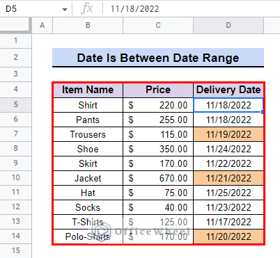
- This is what the table looks like:
Read More: Highlight Row If Cell Contains Text with Conditional Formatting in Google Sheets
Conclusion
In this article, we showed you how to highlight row based on a date in Google Sheets in two methods. We hope this article was useful to you. Keep practicing the methods we have shown here to better understand the concept.
Also, check out other articles on OfficeWheel to keep on improving your Google Sheets work knowledge.
Related Articles
- How to Highlight Highest Value in Row in Google Sheets (2 Ways)
- Use REGEXMATCH Function for Multiple Criteria in Google Sheets]
- How to Use Multiple IF Statements in Google Sheets (5 Examples)
- Use Nested IF Function in Google Sheets (4 Helpful Ways)
- How to Use IF and OR Formula in Google Sheets (2 Examples)
- Filter Values that Contains Multiple Text Criteria in Google Sheets (2 Easy Ways)
- Use IF Condition Between Two Numbers in Google Sheets