Google Sheets: Highlight Row If Cell Is Empty

When working with larger databases, it might be difficult for human eyes to spot all the flaws or gaps. We can be a little bit smarter and lessen the strain on our eyes If we utilize the function or formulas of Google Sheets to highlight row if the cell is empty. Below are a few simple strategies.

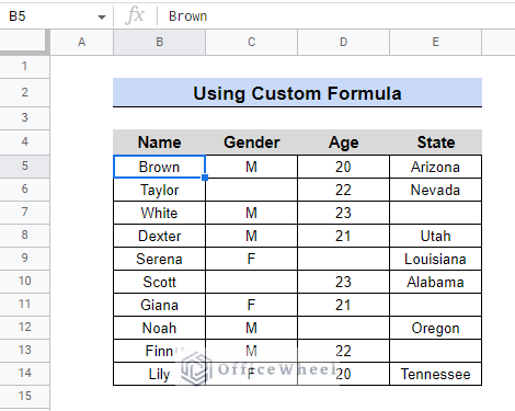
A Sample of Practice Spreadsheet

3 Strategies to Highlight Rows If Cell Is Empty in Google Sheets

There are 3 approaches we can take to highlight a row if a cell is empty in Google Sheets. Each has a special function and formula, but the general procedure is the same in all circumstances. Conditional formatting will make the process look easier. To explain each scenario, we’ll make use of a simple dataset.

1. Using Custom Formula

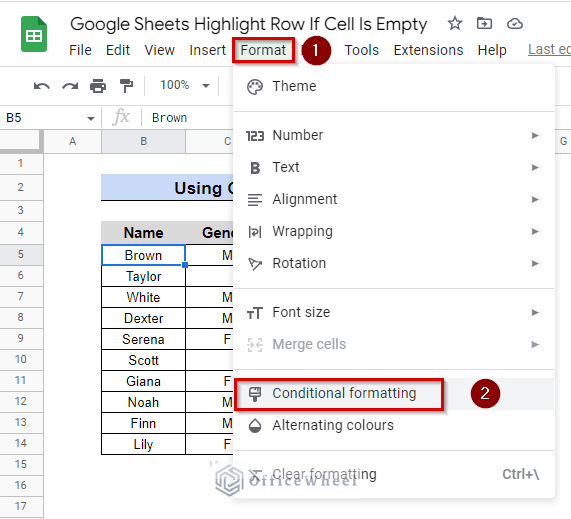
We must first open the Conditional formatting window before we can utilize the custom formula. The following are the steps.

Steps:

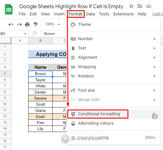
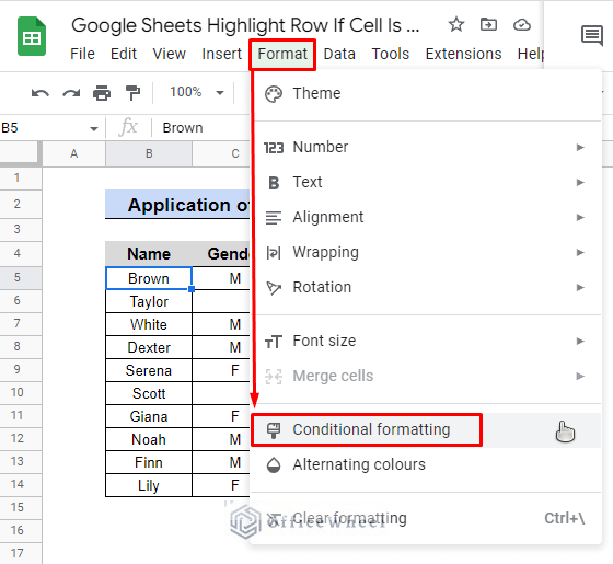
• First, select the Format option from the ribbon.
• Next, choose Conditional formatting from the drop-down.

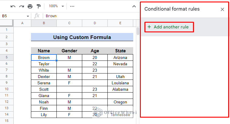
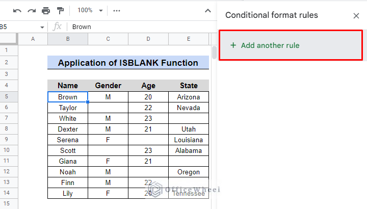
• On the right side of the panel Conditional format rules, a window will appear. Select Add another rule.

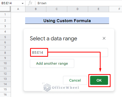
• You will now see a column labeled Conditional format rules. Here, the first step is to simply click the red box in the following image to set the data range.

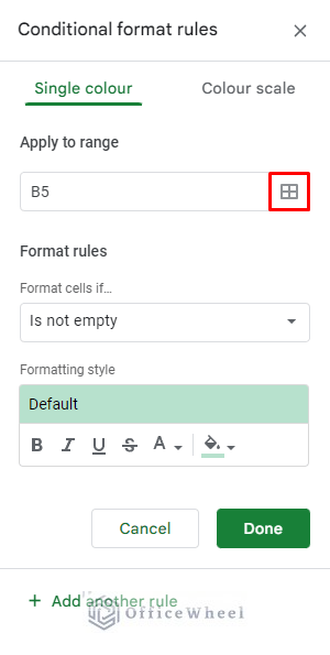
• A new window will appear where you may set the data range, which in this case is B5:E14. Click OK to complete.

• Set the format rules such as that Is Empty > Custom formula is.

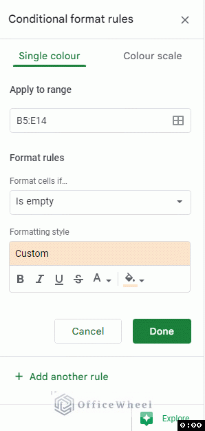
• Immediately underneath the Custom formula is, a little box will show up. Here, we’ll put the custom formula for all that is:

• The $ causes the rule to look at only column C in any row, even if it is evaluating the rule for cells in columns B-E (Which is a part of the whole conditional formatting range). We can say that column C is locked whereas the rows are unlocked.
• To highlight the row, you can use any Fill color. We are utilizing the light orange color in this instance.
• Then click “Done.”

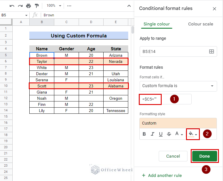
Column C contains two empty cells, as you can see, thus it highlights the two rows.

Read More: Using Conditional Formatting With Custom Formula in Google Sheets

Similar Readings

• Highlight Row If Cell Contains Text with Conditional Formatting in Google Sheets
• How to Copy Conditional Formatting in Google Sheets
• Conditional Formatting Based on Another Cell in Google Sheets
• Highlight Duplicates in Google Sheets (4 Ways)
• Conditional Formatting with Multiple Conditions Using Custom Formulas in Google Sheets

2. Applying the COUNTBLANK Function

Instead of creating a special formula, we’ll take advantage of the COUNTBLANK function to highlight the rows. Same dataset as previously. But in this situation, we’ll focus on column D. The procedures remain unchanged.
Steps:

• Format > Conditional formatting
• Click Add another rule.

• Select data range from B5:E14.
• Establish the formatting rules as Is Empty > Custom formula is.
• Use the following formula:

• Use any Fill color to draw attention to the row. In this case, we’re using light orange same as before.
• Next, select “Done.”

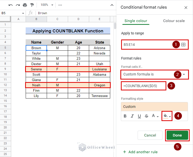
Only two empty cells are present in column D in the figure above. We have highlighted all rows with empty cells using Conditional formatting and the COUNTBLANK function.

Read More: Google Sheets: Conditional Formatting Row Based on Cell

3. Application of ISBLANK Function

Using the ISBLANK function, we can also get the same outcome. We will check column E with this function in order to find any blank cells. Only the formula has changed; all other processes remain the same.
Steps:

• In the beginning, click on Format.
• After that, from the drop-down, select Conditional formatting.

• Click Add another rule.

• Select data range from B5:E14 like before.
• Again, Establish the formatting rules as Is Empty > Custom formula is.
• Use the following formula:

• Choose any Fill color.
• Finally, select “Done”.

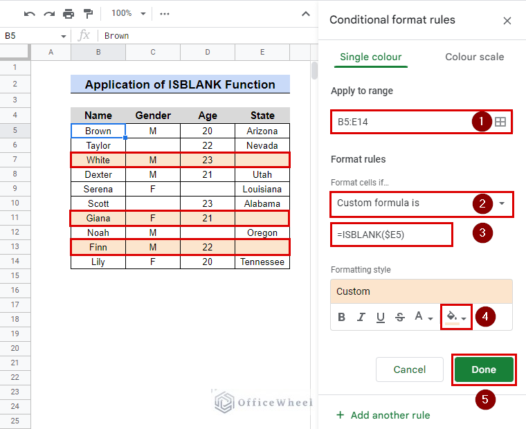
It is clear that column E has three empty cells. The ISBLANK function identifies the cells, and Conditional formatting allows us to highlight the entire row.

Read More: Change Row Color Based on Cell Value in Google Sheets (4 Ways)

Conclusion

Using conditional formatting in Google Sheets allows you to format cells differently depending on whether or not certain criteria are met. When it comes to highlighting rows when a cell is empty, conditional formatting is really beneficial. Within seconds, it simplified human tasks. Check out OfficeWheel‘s blog for additional cool shortcut tricks now that you know how to highlight rows when there are empty cells.

Related Articles

• How to Search in All Sheets in Google Sheets (An Easy Guide)
• Highlight Duplicates in Two Columns in Google Sheets (2 Ways)
• Pivot Table Formatting in Google Sheets (3 Easy Ways)
• Copy Formatting From One Sheet To Another In Google Sheets (2 Ways)
• Conditional Formatting with Checkbox in Google Sheets
• Google Sheets: Conditional Formatting with Multiple Conditions
• How to Highlight Duplicates for Multiple Columns in Google Sheets