Sometimes while working on a spreadsheet we have to highlight some rows or columns as per requirement. For example, if you highlight the highest values in your dataset, then it will help you to understand or visualize your required data very easily. In this article, we will demonstrate how to highlight the highest value of a row in google sheets.
A Sample of Practice Spreadsheet
2 Simple Ways to Highlight Highest Value in Row in Google Sheets
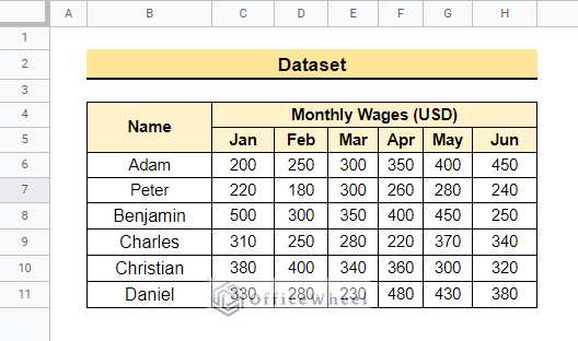
The dataset below contains Name, Monthly Wages (USD), and represents the wages these workers get every month for the last 6 months. Now we will highlight the highest wages they get every month for each person.
Follow the methods below to highlight the highest value in each row using Conditional formatting in Google Sheets.
1. Applying Conditional Formatting with MAX function
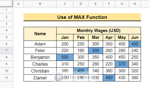
Here, we will apply conditional formatting with the MAX function to highlight the highest value in each row using the following dataset. The MAX function returns the highest value in the given range.
📌 Steps:
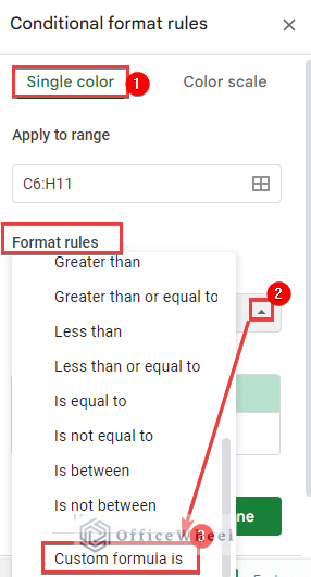
- First, select the cell range C6:H11 to apply conditional formatting.

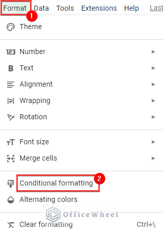
- Then select Format, and you will find the conditional formatting option from the drop-down list.
- After that, the “conditional format rules” window will pop up.
- As the range is already selected, then we will select the drop-down button of “Format rules” and select “Custom formula is” like the following picture.
- After that, we will insert the formula into the “ Value or Formula” box. Then we will choose a color from the Formatting style and click on Done.
=C6=MAX($C6:$H6)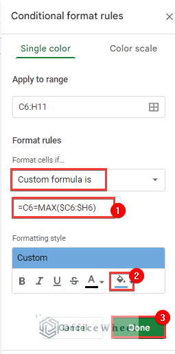
- At last, the output will be like below.
Read More: Highlight Row If Cell Contains Text with Conditional Formatting in Google Sheets
Similar Readings
- How to Highlight Row If Cell Is Not Empty in Google Sheets
- Highlight a Row If Date in Cell Is Today in Google Sheets
2. Utilizing LARGE Function with Conditional Formatting
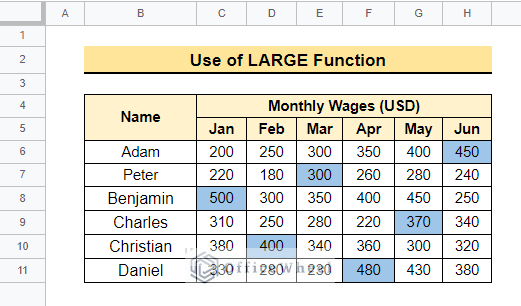
We can also use the LARGE function to highlight the highest value in each row in the same dataset. The LARGE function returns the largest value in a range of numbers.
📌 Steps:
- First, select the cell range C6:H11 to highlight the highest value.
- Then select Format >> Conditional formatting as before.
- After the “Conditional format rules” window will pop up we will select “Custom formula is” from “Format rules” and insert the following formula into the “ Value or Formula” box.
=C6>=LARGE($C6:$H6,1)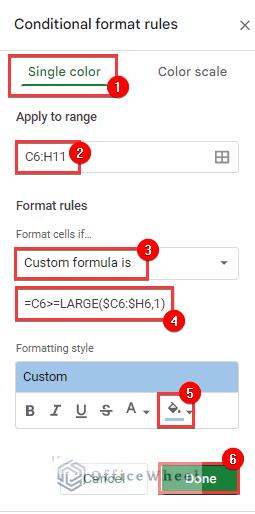
- After clicking Done the output will be like the below.
Read More: How to Highlight a Row in Google Sheets (3 Quick Methods)
How to Highlight Lowest Value in Row in Google Sheets
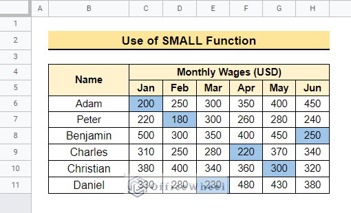
We can also highlight the lowest value in a row in google sheets. In that case, we have to change the formula to the SMALL function.
- We can apply conditional formatting with the SMALL function using the formula below in conditional formatting.
=C6<=SMALL($C6:$H6,1)- Then, the lowest values in each row will be highlighted as follows.
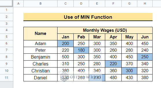
- We can also apply conditional formatting with the MIN function to highlight the lowest data using the below formula in conditional formatting.
=C6=MIN($C6:$H6)- Then, the output will be the same as earlier.
Read More: Highlight Lowest Value in Row in Google Sheets (2 Easy Ways)
Things to Remember
- Always lock the cells while applying the formulas in conditional formatting.
- You can add another formula using Add another rule in conditional formatting.
Conclusion
In this article, we learn how to highlight the highest values in each row in Google Sheets using conditional formatting with different formulas. Hopefully, the methods will help you to apply the function to your own dataset. Please let us know in the comment section if you have any further queries or suggestions. You may also visit our OfficeWheel blog to explore more Google Sheets-related articles.