Filter Values that Contains Multiple Text Criteria in Google Sheets (2 Easy Ways)

Filtering in Google Sheets is a core process required by most analysts. While there are a plethora of great filter conditions already available in Google Sheets, sometimes user requirements call for an expert touch.

One such situation is when we are asked to filter entries that follow the “contains multiple text” criterion in a Google Sheets worksheet.

We have two ways available in our arsenal, both of which require some knowledge of formula creation.

Let’s have a look.

2 Ways to Filter Entries for the Contains Multiple Text Criterion in Google Sheets

The “contains multiple text” criterion strictly means that a cell value has all of the multiple text conditions present. This calls for the AND logical condition which the following methods will use.

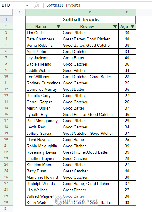
The scenario: Filter entries where the Review column contains both “Good” and “Pitcher” texts.

1. Setting Up a Custom Formula in the AND logic in Google Sheets Filter

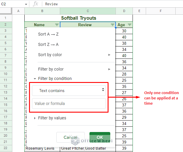
While it is possible to filter for the “contains text” in Google Sheets by default, the filter cannot take more than one value at a time in a single column.

To remedy this, we must resort to creating a custom formula that satisfies the user’s requirements. This custom formula is based on two conditions:

1. A text match. This can be done with the help of regular expression, namely by using the REGEXMATCH function.
2. The AND logical condition. Both text matches must be TRUE.

Step 1: We must first create the custom formula that we will apply to the filter. This is another way for us to understand how the conditions can be brought together in a single formula.

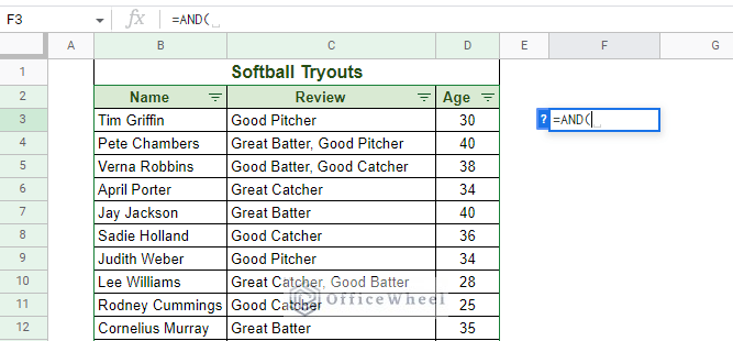
To start, we open the AND function to make the conditions act in the AND logic.

Step 2: Apply the two conditions for multiple texts. For this, we use the REGEXMATCH function.

To match the text “Good” we have:

And for “Pitcher” we have:

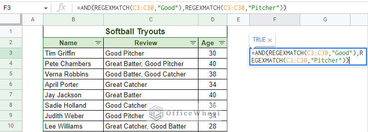
Step 3: Close parentheses and press ENTER. You can use the fill handle to check each row.

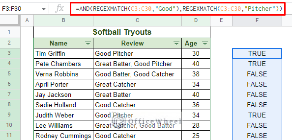
This is the custom formula that we will apply to the filter.

Step 4: Apply this formula in the “Custom formula is” field in the Google Sheets filter menu of the Review column.

Filter > Filter by condition > Custom formula is > Input custom formula

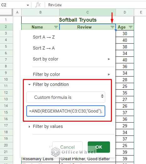
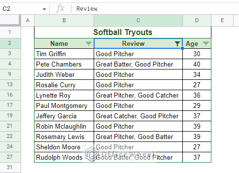
Step 5: Click on OK to apply the filter for multiple “Contains text” criteria in Google Sheets.

Alternatively, you can also use the asterisk or multiplication symbol (*) instead of using the AND function to apply the AND logic. The formula:

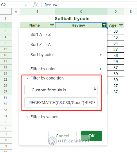
Read More: How to Filter by Condition Using a Custom Formula in Google Sheets (3 Easy Examples)

2. Using the FILTER function for Contains Multiple Text Criterion in Google Sheets (Separate Location/Worksheet)

The second method for filtering for multiple “text contains” criteria in Google Sheets uses the FILTER function.

The function is amazing for its customizability for conditions and comes with a few other advantages that we will see shortly.

As a function, FILTER presents data separately in the worksheet or a separate worksheet.

Step 1: Open the FILTER function at the desired location. For this example, we will present the filtered data in a separate worksheet.

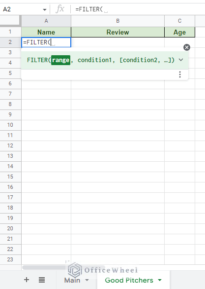
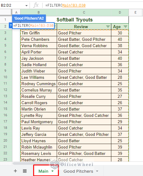
Step 2: Apply the data range of the source dataset.

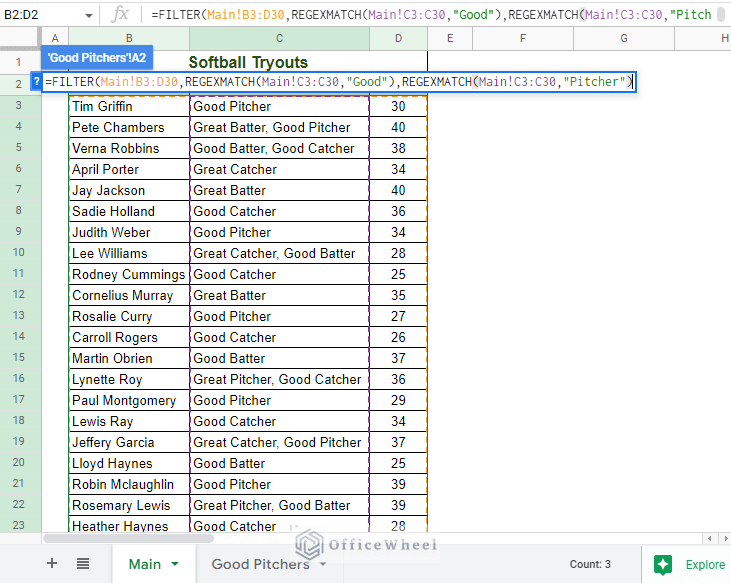
Step 3: Apply the two text conditions. They will once again be the REGEXMATCH formulas that we’ve used previously. Separate the two conditions with a comma since the FILTER function utilizes the AND logic by default:

Step 4: Close parentheses and press ENTER. You will be taken to the worksheet with the FILTER function that has the results.

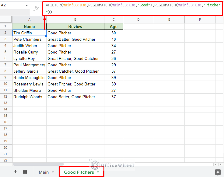
Note: The FILTER formula is not confined to having the conditions in a single column. It can work with multiple columns as well since the condition fields are separate.

Read More: Filter Values that Contains Multiple Text Criteria in Google Sheets (2 Easy Ways)

Similar Readings

• How to Filter with the OR Condition in Google Sheets (3 Easy Ways)
• Google Sheets: Conditional Formatting Row Based on Cell
• How to Filter for Multiple Conditions in Google Sheets (2 Easy Ways)
• How to Find and Replace Blank Cells in Google Sheets
• How to Filter by Condition Using a Custom Formula in Google Sheets (3 Easy Examples)

Filter for Does Not Contain Multiple Text Criterion

We can also opt to filter for the opposite condition, that is filter for entries that “does not contain multiple text” criterion in Google Sheets.

All we have to do is transform the previously generated custom formulas to their opposite values. Simply put, just put it through a NOT logical condition.

For example, to change the filter custom formula to show entries except “Good” and “Pitcher”, all we must do is add an “=FALSE” condition after the criteria (REGEXMATCH).

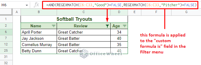
And as for the FILTER formula, we once again set the condition to FALSE for the REGEXMATCH criteria:

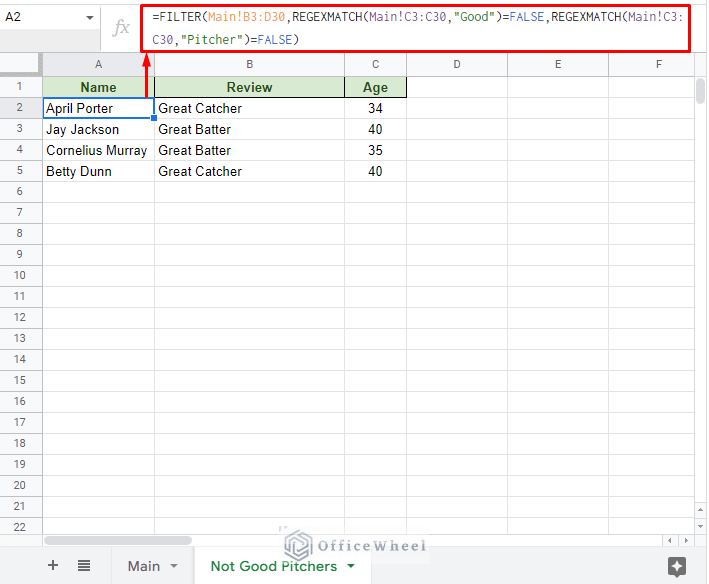
Read More: Google Sheets: Filter for Multiple Criteria with Formula (2 Easy Ways)

Final Words

With the correct understanding of logical formulas, it can be quite easy to filter values that follow the “contains multiple text” criterion in Google Sheets.

If you are using the default filter feature of Google Sheets then it is crucial to generate a custom formula for the condition. Otherwise, for the FILTER function, you can apply and present the filter condition anywhere, whether it is the same or a different worksheet.

Feel free to leave any queries or advice you might have for us in the comments section below.

Related Articles

• How to Do IF THEN in Google Sheets (3 Ideal Examples)
• Use IF and OR Formula in Google Sheets (2 Examples)
• How to Use Multiple IF Statements in Google Sheets (5 Examples)
• Google Sheets: Conditional Formatting with Multiple Conditions
• How to Set a Filter in Google Sheets (An Easy Guide)
• Use Nested IF Function in Google Sheets (4 Helpful Ways)
  
• Google Sheets: Filter Data that Contains Text (3 Easy Ways)
• How to Create Filter Views in Google Sheets (An Easy Guide)