If we’re talking about developing a financial model for business forecasting, Google Sheets excels without a doubt. When undertaking financial modeling, it is essential to use the IF function to create conditional scenarios. You may learn the fundamentals of using the IF function in Google Sheets between two numbers by reading this article.
A Sample of Practice Spreadsheet
You can copy our spreadsheet that we’ve used to prepare this article.
3 Simple Ways to Use IF Condition Between Two Numbers in Google Sheets
The IF function is required to construct conditional situations. There are, however, alternative methods. In the part that follows, we’ll list each one individually.
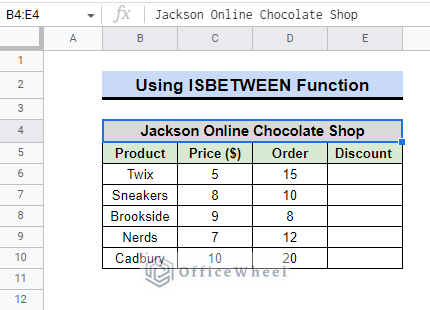
Assume that an online chocolate store decided to offer discounts based on the cost of the product and the size of the order. Data about a few orders are available. To demonstrate all the options, we shall use this simple example.
1. Use of ISBETWEEN Function
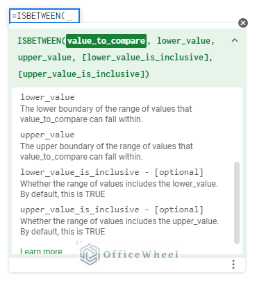
The ISBETWEEN function, in contrast to the IF function, only compares the values between two numbers—one is lower value and the other is upper value—and then returns in boolean form. TRUE if the conditions are met; FALSE if they are not. Take a look at the examples below.
I. Between Two Numbers
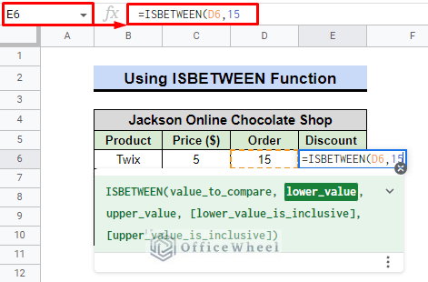
Assume that if the order is between 15 and 30, the store will offer a 10% discount. Using the ISBETWEEN function, we’ll determine whether they qualify. It should be noted that the value must be lower than the upper limit and higher than the lower limit.
Steps:
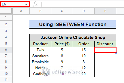
- Select cell E6 first.
- After that, type ISBETWEEN in the formula bar.
- Select the cell or value to compare, for this case it’s E6.
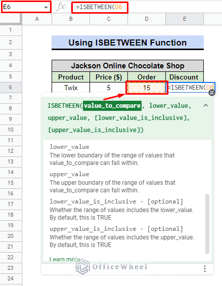
- We will select 15 as the lower value.
- As the upper limit, we will take 30.
- The following logical statement determines whether the lower number is part of the range of values or not. Despite being optional, This is by default TRUE. It will be FALSE since we don’t want to include the lower value.
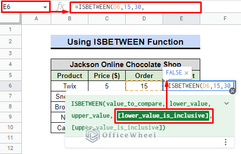
- Additionally, the highest limit is also optional. As we don’t want to include the upper value, it is also FALSE.
- To see the result, press ENTER at the very end.
=ISBETWEEN(D6,15,30,FALSE,FALSE)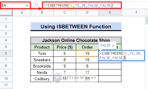
- Google sheets will automatically display a Suggested auto-fill.
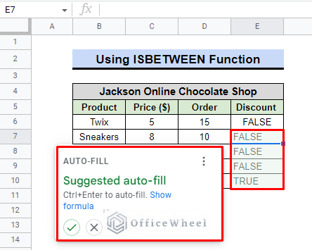
- Click the “✔” to confirm.
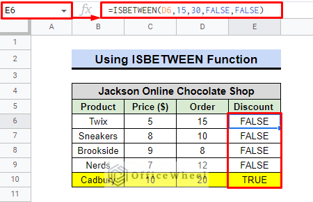
As it turns out, only one order—the one from Cadbury—is qualified for the discount.
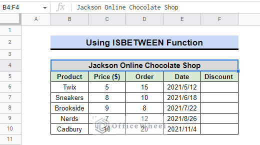
II. Between Two Dates (Considering Date as a Number)
Think about the fact that the store will give a 10% discount on every order placed between May and June of 2021. Now we are going to use the IF condition between two numbers in Google sheets.
Steps:
- We shall once more choose cell E6.
- Following that, we’ll utilize the formula.
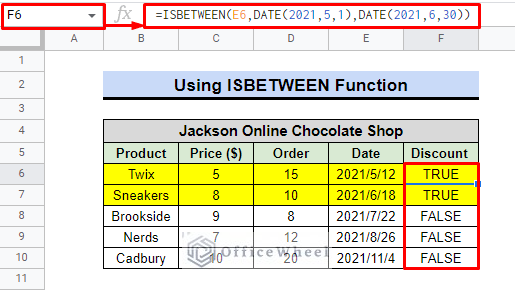
=ISBETWEEN(E6,DATE(2021,5,1),DATE(2021,6,30))- See the outcome by pressing ENTER.
Formula Breakdown:
- E6 is the value with which to compare.
- (2021,5,1) as (YYYY,MM,DD) to represent the date with the help of the DATE function as the lowest limit.
- (2021,6,30) as (YYYY,MM,DD) to denote the date with the aid of the DATE function as the upper limit.
As a result of being ordered on time, the Twix and Sneakers orders will receive a 10% discount.
Read More: How to Calculate Hours Between Two Times in Google Sheets
Similar Readings
- Calculate Number of Years Between Two Dates in Google Sheets
- Difference Between COUNT and COUNTA in Google Sheets
- Google Sheets Count Cells Between Two Numbers with COUNTIF Function
- How to Find Correlation Between Two Columns in Google Sheets
- Insert Rows Between Other Rows in Google Sheets (4 Easy Ways)
2. Utilize IF and AND Functions
Consider that the store wants to offer a 10% discount if the order of the product is greater than or equal to 15 and lesser than or equal to 20, or a 5% discount in all other circumstances.
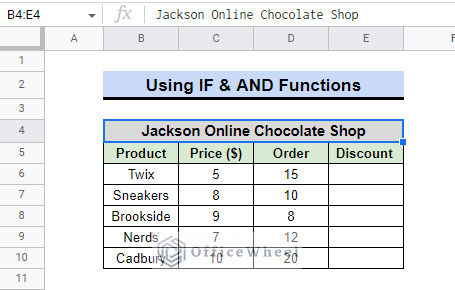
Using the IF and AND functions together, we can determine which order will receive what kind of discounts. To create conditional arguments with numbers as values, we can use the IF function. We will be using the AND function to ensure all the logical expressions are TRUE. Follow the steps below to understand the concept.
Steps:
- We will choose cell E6 initially.
- Next, we’ll add the following formula:
=IF(AND(D6>=15,D6<=20),"10%","5%")- To see the outcome, press ENTER.
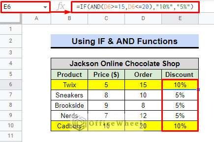
Formula Breakdown:
- The logical arguments for the AND function are (D6>=15, D6<=20). It states that the value of D6 should be between 15 and 20 or equal to it.
- If the AND function returned TRUE for the logical statement, “10%” will be displayed as value_if_true.
- The IF function will display “5%” if the AND function returns FALSE for any of the arguments.
We shall discover that only two orders, Twix & Cadbury, may satisfy the first requirements. 5% off the remainder of the orders.
Read More: How to Calculate Time Between Dates in Google Sheets (6 Ways)
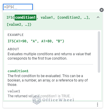
3. Application IFS Function
We can utilize the IFS function to add extra numerical criteria. The IFS function analyzes many criteria and returns a result that is equal to the first true condition.
Consider the scenario where the store provides two distinct discounts. One is 15%, which requires a price greater than or equal to $8 and lesser than $10. Another is a 20% discount if the entire order is between 15 and 20, or equal to it.
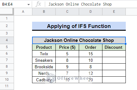
If the order doesn’t qualify for either of the two discounts, the store won’t provide any discount. To resolve this scenario, we will use the IFERROR function. Check out the instructions below.
Steps:
- First, we will select cell E6.
- Then, enter the following formula
=IFERROR(IFS(AND(C6>=8,C6<=10),"15%",AND(D6>=15,D6<=20),"20%"),"0%")- Press ENTER once more to finish.
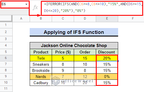
Formula Breakdown:
- The arguments of the AND function to verify first are (C6>=8,C6<=10) which states that C6 should have a value of 15 or greater but not greater than 20.
- The IF function will display “15%” if the value returned by the AND function is TRUE.
- The following arguments (D6>=15, D6=20), which specify that the value of D6 should be equal to or between 15 and 20, will be examined if the AND Function returns a FALSE value.
- Again, the IF function will show “20%” if the return result from the AND function is TRUE.
- Finally, IFERROR will return “0%” as the result of the error if both parameters return FALSE values when tested with the AND function.
We’ll get an intriguing result because only one order, Twix, will get discounts of 20%. Conversely, 15% off will be given on orders for Sneakers, Brookside and Cadbury. One order will, however, not be eligible for any discounts.
Read More: Calculate Percentage Difference Between Two Numbers in Google Sheets
Final Words
When working with big data, we frequently come across conditional circumstances. In Google Sheets, depending on the circumstance, we can utilize the IF or ISBETWEEN function to distinguish between two numbers or dates. Please leave a comment if you have any questions. For further details, please visit OfficeWheel.
Related Articles
- Remove Spaces Between Words in Google Sheets
- How to Filter Between Two Dates in Google Sheets
- Generate Random Numbers or Text Between Limits in Google Sheets
- Find Number of Months Between Two Dates in Google Sheets
- How to Find Missing Values Between Two Columns in Google Sheets
- Conditional Formatting Between Two Values in Google Sheets
- How to SUMIF Between Two Dates in Google Sheets (3 Ways)