The AND function is a very much popular function in Google Sheets. We can use this function to get logical output on a set of conditions. The AND function can be used alone and also with different functions like the IF and OR functions. In this article, I’ll show 4 suitable examples to use AND function in Google Sheets with clear steps and images.
A Sample of Practice Spreadsheet
You can download Google Sheets from here and practice very quickly.
What Is AND Function in Google Sheets?
The AND function in Google Sheets gives TRUE if all the conditions are true otherwise FALSE.
Syntax
The syntax of the AND function is like below-
AND(logical_expression1, [logical_expression2, …])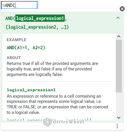
Argument
| Argument | Requirement | Function |
|---|---|---|
| Logical expression 1 | Required | Reference or text containing the logic |
| Logical expression 2 | Required | Extra reference or text containing the logic |
Output
The formula AND(A1=1, A2=2) will show TRUE as output if both conditions are matching otherwise FALSE.
4 Suitable Examples to Use AND Function in Google Sheets
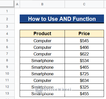
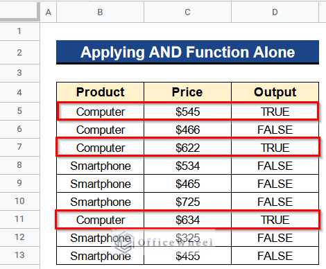
Let’s get introduced to our dataset first. Here we have 2 common products, i.e. Computers and Smartphones in Column B and their prices in Column C. Now we’ll see how to use the AND function in Google Sheets to set different criteria with this dataset.
Example 1. Applying AND Function Alone
The AND function is self-sufficient. We can use this function alone with different criteria. In this example, we want to get TRUE if the product is Computer and its price is above $500. Let’s see how to do it.
Steps:
- Firstly, type the following formula in Cell D5–
=AND(B5 = "Computer" ,C5 > 500)- Secondly, hit Enter to get the output.
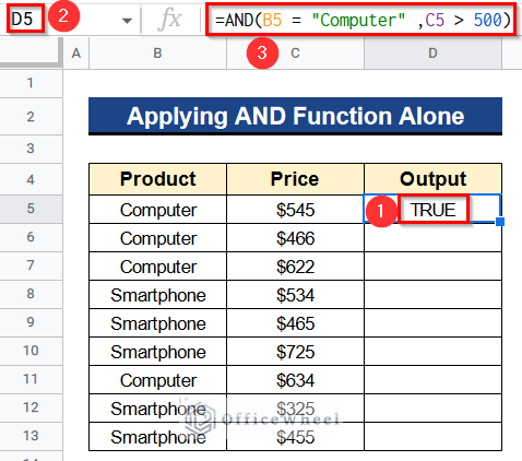
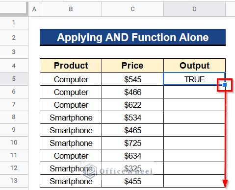
- Finally, you’ll get TRUE for those Computers whose prices are higher than $500 otherwise FALSE.
Read More: Conditional Formatting with Multiple Conditions Using Custom Formulas in Google Sheets
Example 2. Using AND Function with Helper Column
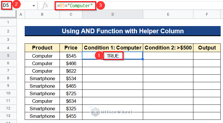
We can also use the AND function with the help of creating helper columns. Now we want the same output as Example 1. But this time we’ll make 2 helper columns and then apply the AND function with respect to these columns. This process is a bit lengthy.
Steps:
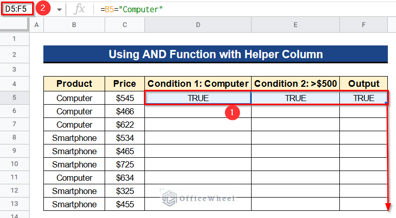
- At first, write the following formula in Cell D5–
=B5="Computer"- Then, press Enter to get the result.
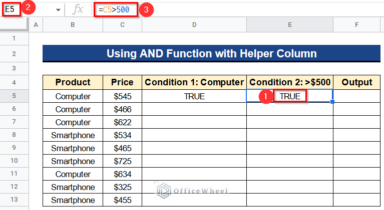
- Again, insert the below formula in Cell E5–
=C5>500- Next, hit the Enter Button to get your desired output.
- At last, put the next formula in Cell F5–
=AND(D5,E5)- Ultimately, press the Enter Button to get the final result.
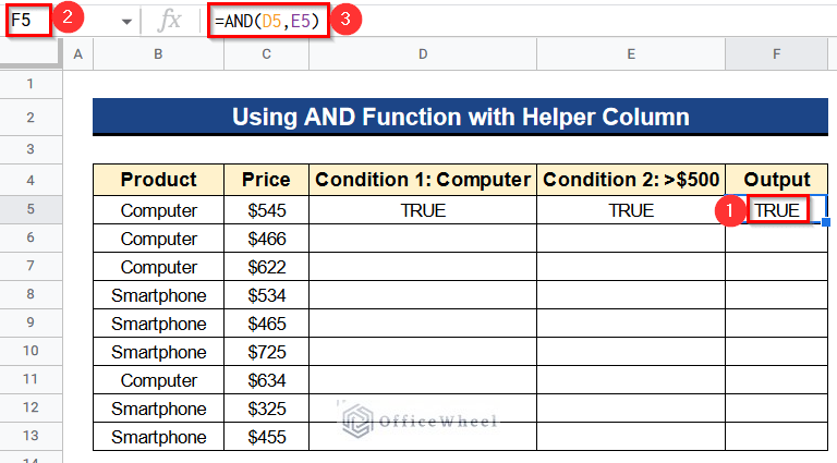
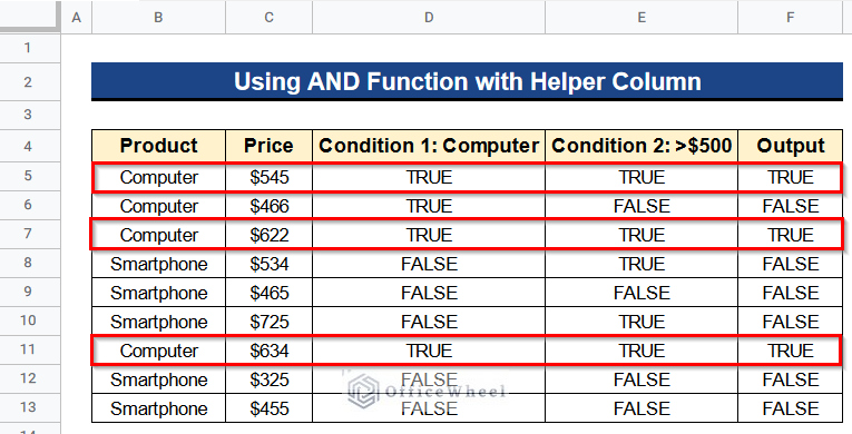
- Moreover, select Cells D5 to F5 together and apply the Fill Handle tool.
- In the end, the final result will be like the following picture. It’ll give TRUE if conditions are met or otherwise FALSE as you can see in the picture.
Read More: Google Sheets: Conditional Formatting with Multiple Conditions
Similar Readings
- How to Use ARRAYFORMULA with IF Function in Google Sheets
- Highlight Row If Cell Is Not Empty in Google Sheets
- Highlight Row Based on Date in Google Sheets (2 Suitable Ways)
- Filter Values that Contains Multiple Text Criteria in Google Sheets (2 Easy Ways)
- Find if Date is Between Dates in Google Sheets (An Easy Guide)
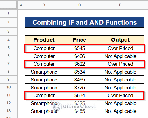
Example 3. Combining IF and AND Functions
Now we don’t want the output as TRUE or FALSE. If the product is a Computer and its price is above $500, then we want the output as Over Priced. And If the condition doesn’t match then we want Not Applicable as our output. We can simply do this by combining the IF and AND functions together.
Steps:
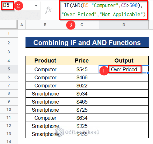
- First of all, type the following formula in Cell D5–
=IF(AND(B5="Computer",C5>500), "Over Priced","Not Applicable")- Consequently, hit Enter to get the output.
Formula Breakdown
- AND(B5=”Computer”,C5>500)
Before all, this function will search for Computer in Cell B5 and values greater than 500 in Cell C5. Finally, it returns TRUE if both conditions are met otherwise FALSE.
- IF(AND(B5=”Computer”,C5>500), “Over Priced”,”Not Applicable”)
Then, this function will give Over Priced for the condition met with the help of the AND function. If the condition doesn’t match then it’ll give Not Applicable.
- Thereafter, assign the Fill Handle tool to apply the formula in Column D.
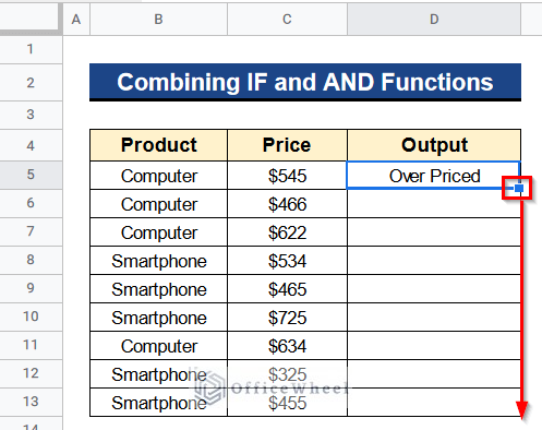
- Afterward, you’ll get Over Priced in the cells if the condition is met and Not Applicable in the rest of the cells.
Read More: How to Use IF Function in Google Sheets (6 Suitable Examples)
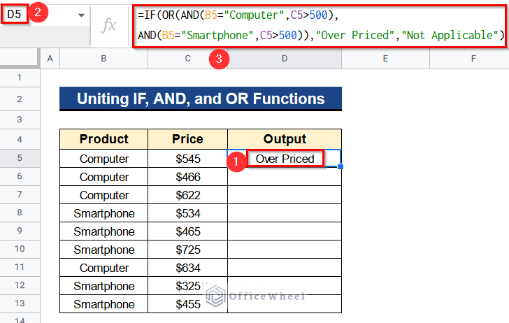
Example 4. Uniting IF, AND, and OR Functions
This time we’ll unite the IF, AND, and OR functions together to extend our conditions. Besides getting the output for computers priced above $500 we now want the same result for smartphones also. The steps are given below.
Steps:
- In the first place, write the next formula in Cell D5–
=IF(OR(AND(B5="Computer",C5>500), AND(B5="Smartphone",C5>500)),"Over Priced","Not Applicable")- Then, click on the Enter Button to get your desired result.
Formula Breakdown
- AND(B5=”Computer”,C5>500)
Firstly, this function will search for Computer in Cell B5 and values greater than 500 in Cell C5. Secondly, it returns TRUE if both conditions are met otherwise FALSE.
- AND(B5=”Smartphone”,C5>500)
This function also does the same task as mentioned before. The difference is that now the criteria for searching is Smartphone and values greater than 500.
- OR(AND(B5=”Computer”,C5>500), AND(B5=”Smartphone”,C5>500))
After that, the OR function matches both the criteria and returns TRUE if any of them satisfies the condition.
- IF(OR(AND(B5=”Computer”,C5>500), AND(B5=”Smartphone”,C5>500)),”Over Priced”,”Not Applicable”)
Finally, this function will give Over Priced for the conditions met with the help of both the AND and OR functions. If the condition doesn’t match then it’ll give Not Applicable.
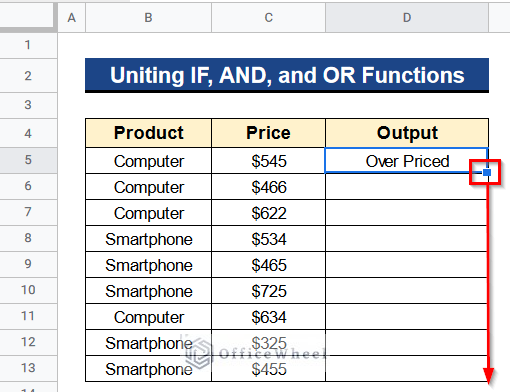
- Later, use the Fill Handle tool to assign the formula in Column D.
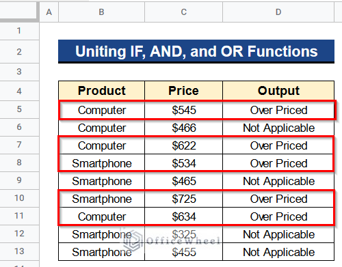
- Ultimately, you’ll get Over Priced in the cells if both conditions are met. Otherwise, you’ll get Not Applicable as you can see in the picture.
Read More: How to Use IF and OR Formula in Google Sheets (2 Examples)
Conclusion
That’s all for now. Thank you for reading this article. In this article, I have discussed 4 suitable examples to use the AND function in Google Sheets. Please comment in the comment section if you have any queries about this article. You will also find different articles related to google sheets on our officewheel.com. Visit the site and explore more.
Related Articles
- How to Do IF THEN in Google Sheets (3 Ideal Examples)
- Use REGEXMATCH Function for Multiple Criteria in Google Sheets
- How to Use Nested IF Function in Google Sheets (4 Helpful Ways)
- Use IF Condition Between Two Numbers in Google Sheets
- How to Use VLOOKUP for Conditional Formatting in Google Sheets
- Use Multiple IF Statements in Google Sheets (5 Examples)
- Match Multiple Values in Google Sheets (An Easy Guide)