Google Sheets has made it much easier for us to work with lots of data and large datasets. Organizing this data properly helps us to read and understand the information effectively. Highlighting every other row is a great way to format and visualize data properly. In this article, we will demonstrate how to highlight every other row in Google Sheets.
A Sample of Practice Spreadsheet
You can download the practice spreadsheet from the download button below.
2 Suitable Ways to Highlight Every Other Row in Google Sheets
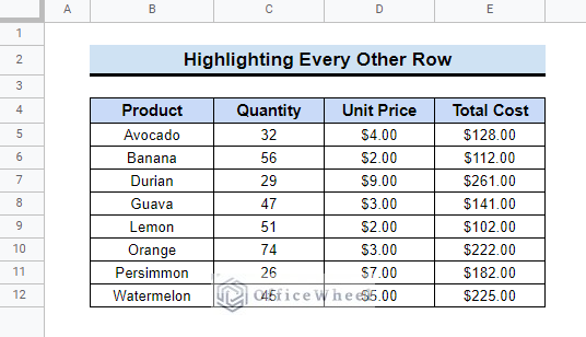
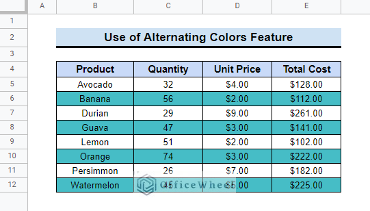
Suppose you have the following dataset containing some products ordered by customers. In this data table, a list of some products, their unit price, purchase quantity, and total cost are mentioned. Now you want to highlight every other row of this table.
 Follow the methods below to see how to do that.
1. Using Alternating Colors Feature
The easiest way to highlight every other row in Google Sheets is to use the Alternating colors feature. It is an awesome built-in feature of Google Sheets. Follow the steps below to learn how to use that to highlight the alternate rows in your dataset.
📌 Steps:
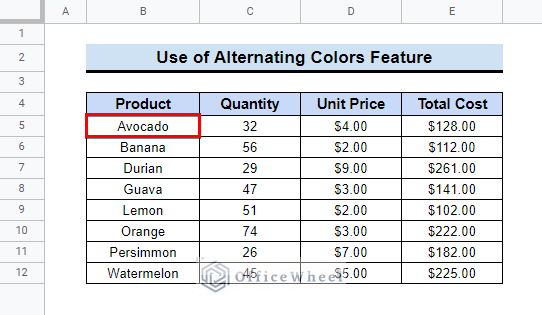
- First, select any cell in the dataset. Here we have selected cell B5. You can also select the entire dataset.
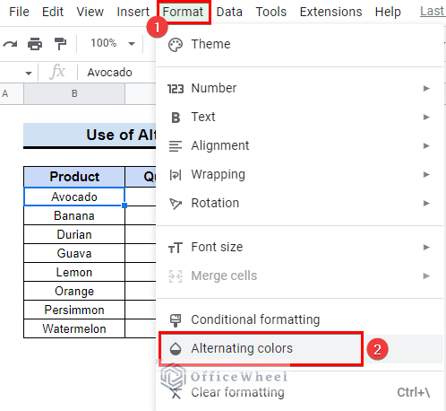
- Next, select the Format tab from the ribbon. Then a dropdown will appear. Now click on Alternating colors from there.
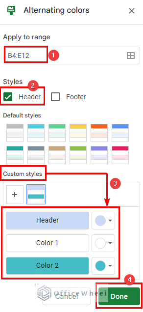
- Then you will see an Alternating colors pane on the right side. Though you selected only one cell, you will see that it has automatically detected the entire range.
- If you select the dataset excluding the headers, you should uncheck the Header checkbox.
- There are some Default styles to choose from. You can also use customized colors from Custom styles. Then click on Done.
- Finally, the table will look like the one below.
Read More: How to Highlight Row If Cell Is Not Empty in Google Sheets
2. Applying Conditional Formatting
Alternatively, you can also apply Conditional formatting to highlight every other row in Google Sheets. Here we will highlight 3 formulas to use in the conditional formatting to get the desired results.
2.1 Using ISODD and ROW Functions
Here we will use the ISODD and ROW functions to create a formula for the conditional formatting. Follow the steps below to be able to do that.
📌 Steps:
- First, select the range B5:E12 (excluding the headers).
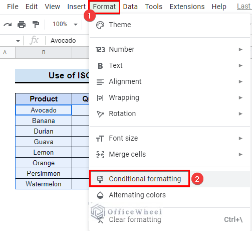
- Then select Format from the ribbon and then select Conditional formatting.
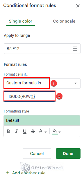
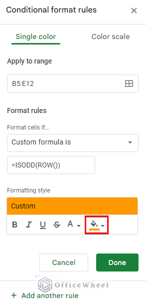
- After that, you will see your selected range in the Apply to range box. Now select Custom formula is from the Format rules dropdown.

- Then insert the following formula in the Value or formula box.
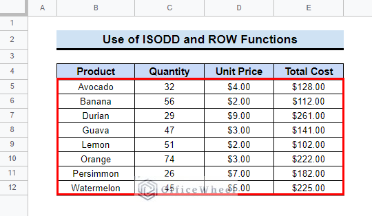
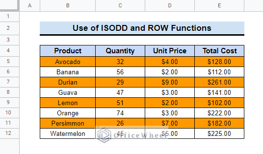
=ISODD(ROW())- The ROW function specifies the row number of a cell and the ISODD function check if the number is odd. These functions together return TRUE for the odd rows.
- After that, choose a color from the Formatting style. You can keep it as Default or select any color from the fill color option.
- Finally, select the Done button. As a result, the data table will look like the following image.
Read More: Highlight Row If Cell Contains Text with Conditional Formatting in Google Sheets
2.2 Applying ISEVEN and ROW Functions
Now we will use the ISEVEN and ROW functions to apply a formula for the conditional formatting. Check the following guideline to learn how to do that.
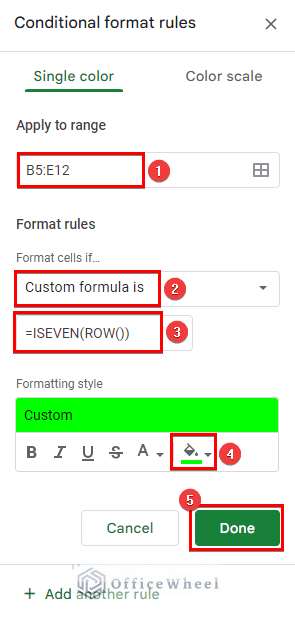
- As in the previous method, select range B5:E12 and go to Format >> Conditional Formatting. Then enter the following formula in the Format rules box.
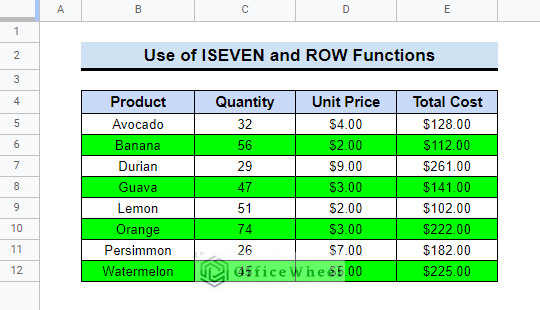
=ISEVEN(ROW())- Here, the ISEVEN function returns TRUE if the row number returned by the ROW function is even. Then the conditional formatting gets applied.
- After that, select any color from the fill color option and press the Done button.
- As a result, the alternate rows will be highlighted as follows.
Read More: Highlight Row Based on Date in Google Sheets (2 Suitable Ways)
2.3 Utilizing MOD and ROW Functions
You can also combine the MOD and ROW functions to create another formula to apply in the conditional formatting. Follow the steps below for that.
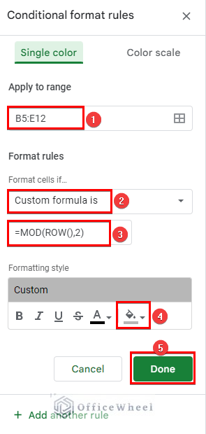
- First, select the range B5:E12 and go to Format >> Conditional Formatting as earlier.
- Then apply the following formula in the formula box for conditional formatting, choose a color and click on Done.
=MOD(ROW(),2)- The MOD function returns the remainder after a number is divided by another. So in this formula, the MOD function will return 1 for the odd rows and 0 for the even rows while dividing by 2. If you want to highlight alternate rows then modify the formula as =MOD(ROW(),2)=0. This will highlight the alternate rows with no remainders.
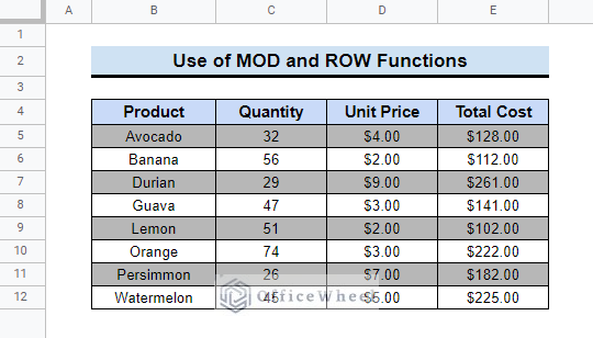
- As a result, you will get the same highlighted data table as given below.
Read More: How to Highlight Active Row in Google Sheets (2 Suitable Ways)
Things to Remember
- If you already have a customized header in the dataset, then you have to select the table range without the header to keep the style while using the Alternating colors feature. Unchecking the header checkbox makes the header color white.
- You can easily copy the conditional formatting to other cells. Just copy any cell with the formatting and use Paste special >> Format only to apply the same formula.
Conclusion
Following the above methods, you can easily highlight every other row in google sheets. This will make your spreadsheet more readable, categorized, and eye-catching. Please use the comment section below for further queries or suggestions. Hopefully, it will help you to visualize your data more properly. You may also visit our OfficeWheel blog to explore more about Google Sheets.