It takes a lot of time to interpret Google Sheets with too much data. One simple solution to this problem is highlighting the important information so it can draw the user’s eye easily. Here, in this article, I’ll be discussing a few methods on how to highlight a row in Google Sheets.
A Sample of Practice Spreadsheet
3 Quick Methods of Highlighting a Row in Google Sheets
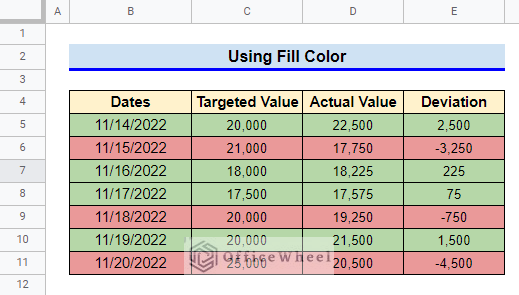
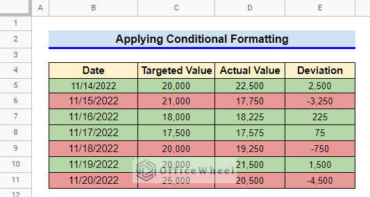
First, we will learn about our datasheet. It contains the Targeted Value, Actual Value, and Deviation of an organization for several dates. We’ll highlight any row with red color that has a negative value of Deviation and will use green color for positive Deviation.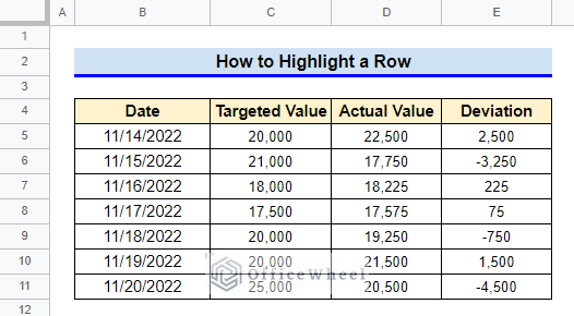
1. Use Fill Color
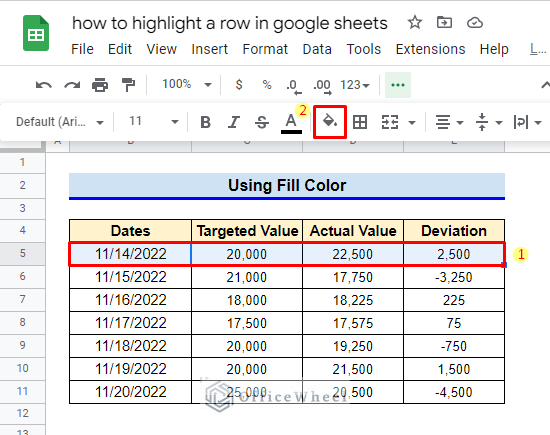
If we want to highlight rows from a dataset that is not very large and doesn’t need to be changed often, we can simply use Fill Color.
Steps:
- First, select the row you want to highlight and then click on the Fill Color option from Clipboard.
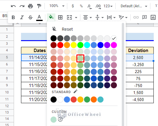
- From the pop-up color options select any color of your choice. I’ll be choosing light green 2 for non-negative values and light red 2 for negative values.
- Thus we have highlighted the required row.
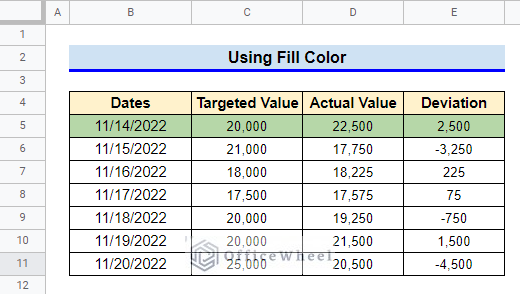
- Repeat the steps for other rows.
Read More: How to Highlight Highest Value in Row in Google Sheets (2 Ways)
2. Apply Conditional Formatting
Using Fill Color to highlight rows in a large dataset can be tedious. Changing the values also doesn’t change the row color if Fill Color is used. To create a more flexible and dynamic datasheet, we can highlight the rows using Conditional Formatting.
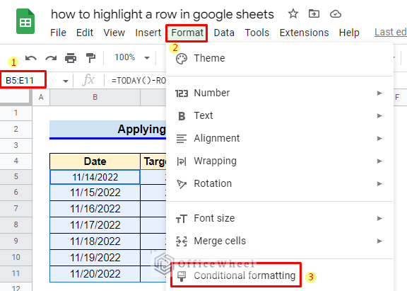
- First, select the rows you want to highlight and then go to the Format Select Conditional Formatting.
- From the pop-up sidebar, click on the dropdown icon Format cells if box.
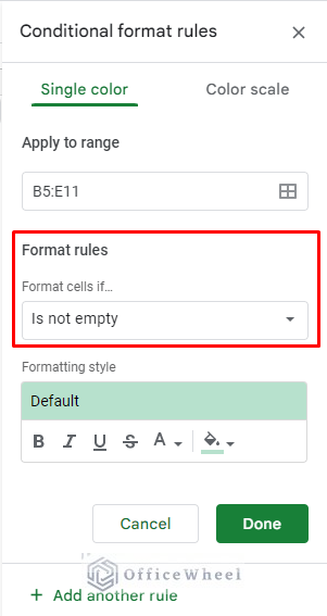
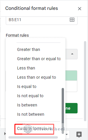
- Select Custom Formula is option from the dropdown options.
- Set the Value or formula in Format Rules as follows. Select light green 2 as Fill Color from Formatting Style, then click on Done.
=$E4:$E11>0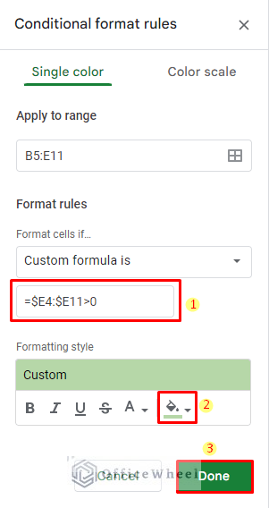
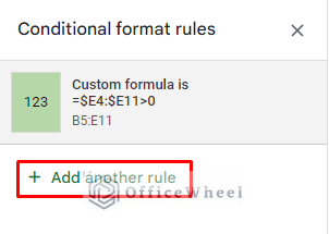
- Now click on +Add another rule.
- Change the custom formula in Format Rules to the following. Also, change the Fill Color to light red 2 in Formatting Style and then click on Done.
=$E4:$E11<0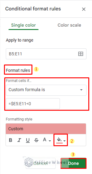
- Thus, we have highlighted the rows in a more flexible and dynamic way.
Read More: Highlight Row If Cell Contains Text with Conditional Formatting in Google Sheets
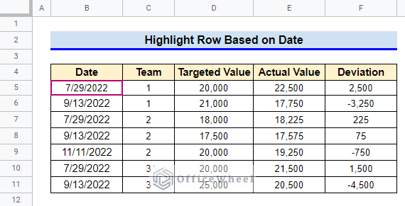
3. Highlight Row Based on Date
In the previous method, we could have highlighted rows based on dates. To demonstrate the process, we have made some changes to our dataset. Firstly, we have changed the dates. Also, we have inserted a new column titled “Team”. So, the dataset now has Targeted Value, Actual Value, and Deviation for different teams on different dates. For this dataset, I’ll highlight the rows with the date 7/29/2022.
Steps:
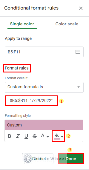
- Follow the first three steps from the previous method to pop up a sidebar like the following. Set the custom formula in Format Rules as follows. Choose any Fill Color according to your requirement from Formatting Style, then click on Done.
=$B5:$B11= “7/29/2022”Note: You will have to keep the dates in Text format for this method.
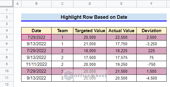
- The rows that include the date 7/29/2022 have been highlighted.
Read More: Highlight Row Based on Date in Google Sheets (2 Suitable Ways)
Things to Be Considered
- For highlighting any row with Custom Formula, you must put the $ symbol in front of the column number. Otherwise, only a single cell from that row will be highlighted instead of the row.
- The dates have to be in Plain Text format while highlighting rows based on dates.
Conclusion
This concludes our article to learn how to highlight a row in Google Sheets. I hope the demonstrated methods were helpful for your requirements. Feel free to leave any comments or advice in the comment box.
Related Articles
- How to Highlight Every Other Row in Google Sheets (2 Methods)
- Google Sheets: Highlight Row If Cell Is Empty
- How to Highlight a Row If Date in Cell Is Today in Google Sheets
- Highlight Lowest Value in Row in Google Sheets (2 Easy Ways)
- How to Highlight Row If Cell Is Not Empty in Google Sheets
- How to Highlight Active Row in Google Sheets (2 Suitable Ways)