We use drop down lists in Google Sheets very often. But sometimes we might find it problematic for updating cell values based on selection in drop down list in Google Spreadsheet. In this article, we’ll show 5 quick and simple methods using some functions and formulas. I hope, it’ll help you solve your problems.
A Sample of Practice Spreadsheet
You can download Google Sheets from here and practice very quickly.
5 Quick Ways of Updating Cell Values Based on Selection in Drop Down List in Google Spreadsheet
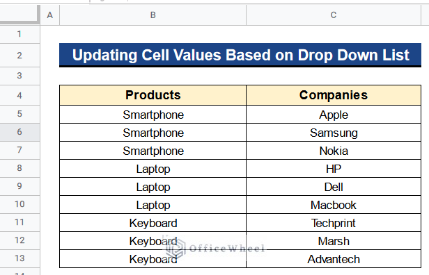
Firstly, let’s get introduced to our dataset. Here we have some products in Column B and their companies in Column C. We’ll make a drop down list of the products and learn how to update the cell values of another drop down list based on the selection in the products’ drop down list in Google Sheets. That’s why we rename this dataset as Datasheet. We’ll use values from this sheet in our methods.
1. Combining UNIQUE, FILTER, and SORT Functions
At first, we’ll do the work by applying the UNIQUE, FILTER, and SORT functions. This method is straightforward. We’ll get the output quickly.
Steps:
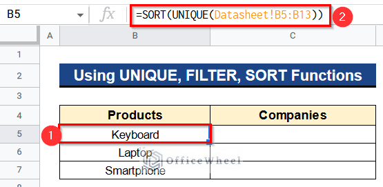
- Type the following formula in Cell B5–
=SORT(UNIQUE(Datasheet!B5:B13))- Hit the Enter to get the unique products list.
Formula Breakdown
- UNIQUE(Datasheet!B5:B13)
This formula searches the unique values and removes the duplicate values from Column B in Datasheet and puts them in the current sheet.
- SORT(UNIQUE(Datasheet!B5:B13))
Finally, it will sort the unique values alphabetically.
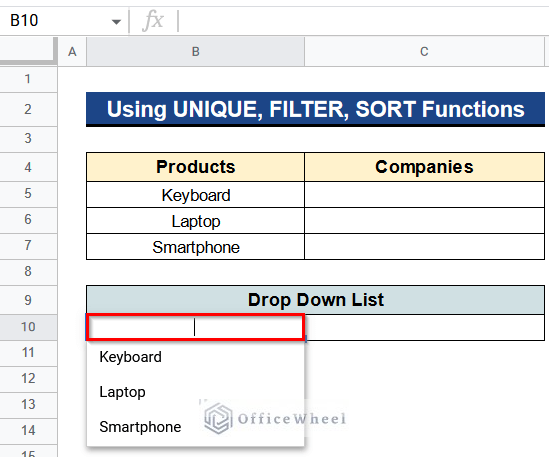
- Now we’ll make a drop down list from the list of unique products.
- Select Cell B10. Go to Data > Data validation.
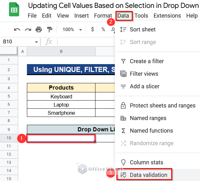
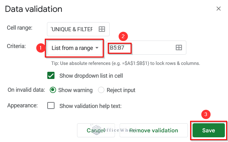
- Select List from a range under the Data validation menu and give the range from B5 to B7 which is our unique product list.
- Then click the Save Button.
- We’ll get a list like this.
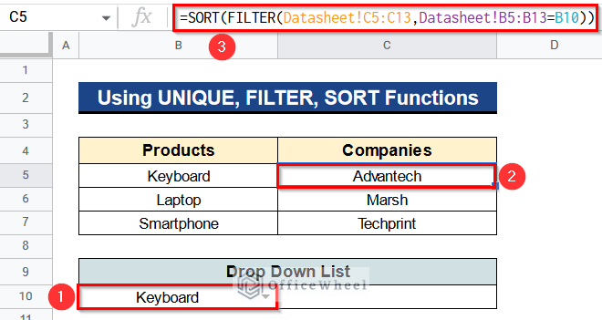
- Type the following formula in Cell C5–
=SORT(FILTER(Datasheet!C5:C13,Datasheet!B5:B13=B10))- Press Enter to get the relevant company name.
Formula Breakdown
- FILTER(Datasheet!C5:C13,Datasheet!B5:B13=B10)
This formula searches for the companies’ names in Column C from the Datasheet corresponding with the selected product value in Column B from the Datasheet and brings the values here.
- SORT(FILTER(Datasheet!C5:C13,Datasheet!B5:B13=B10))
Finally, it will sort the values alphabetically.
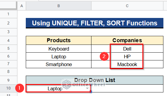
- If you change the product name from the list then the company’s name will automatically get updated.
- Now create a drop down list in Cell C10 with the company’s name by the same procedure.
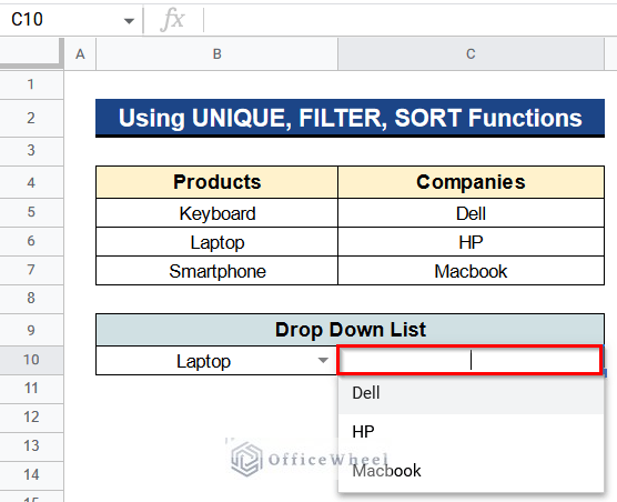
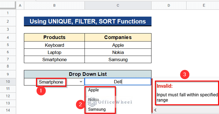
- When we select the product name from the list the adjacent cell shows the company list.
- The Invalid part is shown because we select smartphones in the product list but have a value of other product company names.
- Below you can see the actual list which you can select easily.
Read More: How to Edit Data Validation in Google Sheets (With Easy Steps)
2. Merging IF and QUERY Functions
Now we have a different situation. We want to have the product names in separate columns. Moreover, we want to have the company names under each product in separate columns. And also we want to update it based on the selection in drop down list. In this case, we can use the IF and QUERY functions.
Steps:
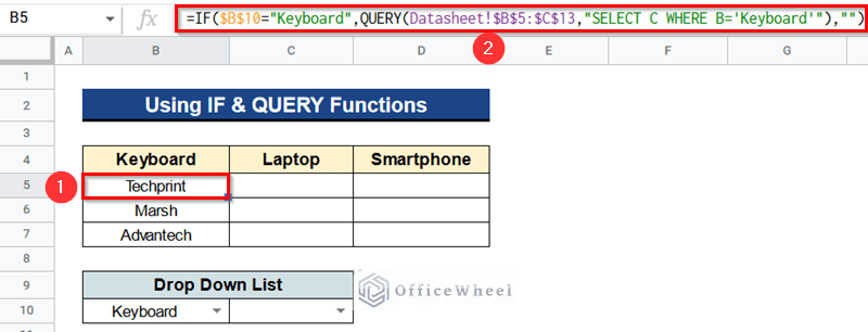
- First, create a drop down list in Cell B10 with the product list in Row 4 following the 3rd, 4th, and 5th steps from the first method.
- Write the following formula in Cell B5–
=IF($B$10="Keyboard",QUERY(Datasheet!$B$5:$C$13,"SELECT C WHERE B='Keyboard'"),"")- Press Enter to get the output.
- Now type the same formula in Cell C5 by changing the formula a little bit-
=IF($B$10="Laptop",QUERY(Datasheet!$B$5:$C$13,"SELECT C WHERE B='Laptop'"),"")- Hit Enter to get the result.

Formula Breakdown
- QUERY(Datasheet!$B$5:$C$13,”SELECT C WHERE B=’Keyboard'”)
This function searches the given value which is ‘Keyboard’ from the Datasheet and from there brings the corresponding value from Column C.
- IF($B$10=”Keyboard”,QUERY(Datasheet!$B$5:$C$13,”SELECT C WHERE B=’Keyboard'”),””)
Finally, it will place the value if it matches with the given logic in this case ‘Keyboard’.
- IF($B$10=”Laptop”,QUERY(Datasheet!$B$5:$C$13,”SELECT C WHERE B=’Laptop'”),””)
This formula also works like the previous formula. But here we have just changed the product name which is ‘Laptop’.
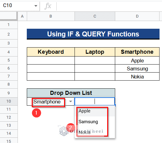
- Do the same action in the next column, Column D which has the smartphone companies list.
- Make a drop down list in Cell C10 using the 3rd, 4th, and 5th steps from the first method.
- And now if you select smartphone from the list you’ll get the corresponding list updated.
Read More: How To Lock Rows In Google Sheets (2 Easy Ways)
Similar Readings
- How to Create Dependent Drop Down List in Google Sheets
- Create Multiple Dependent Drop Down List in Google Sheets
- How to Add Color to Drop Down List in Google Sheets (Easy Steps)
3. Joining INDEX and MATCH Functions
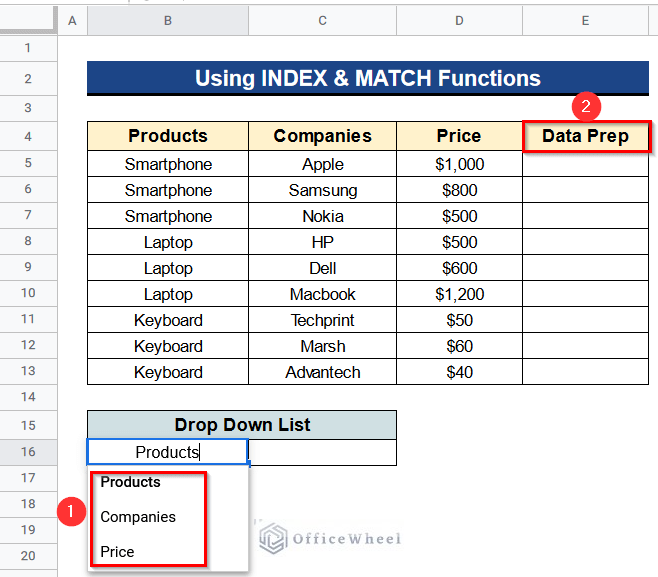
Now we have a dataset with 3 columns which are products in Column B, companies in Column C, and price in Column D. And we have a drop down list below in Cell B16 with the columns header. This time we can solve the problem by using the INDEX and MATCH functions. Firstly, we have to make a Data Prep column in Column E for this purpose.
Steps:
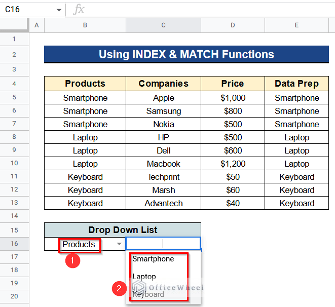
- First, create a drop down list in Cell B16 following the 3rd, 4th, and 5th steps from the first method.
- Write the following formula in Cell E5–
=INDEX(B5:D13,,MATCH(B16,B4:D4,0))- Press Enter to get the result.
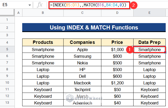
Formula Breakdown
- MATCH(B16,B4:D4,0)
This function searches for the selected product in the drop down list which is in Cell B16. Then it searches for its relative position in Columns B, C, and D.
- INDEX(B5:D13,,MATCH(B16,B4:D4,0))
Finally, it gives the matching values within the data range from Cell B5 to D13.
- Again make another drop down list in Cell C16 by the 3rd, 4th, and 5th steps from the first method.
- . Now, you can select any option from the list and get the updated values as shown in the image.
Read More: Dependent Drop Down List for Entire Column in Google Sheets
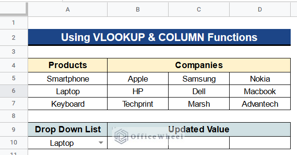
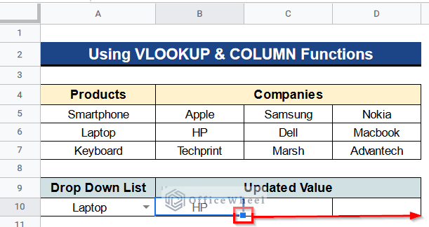
4. Combining VLOOKUP and COLUMN Functions
Again we have a different scenario. Now we have the product’s name in Column A and the company’s name through Column B to Column D. Moreover, we have a drop down list in Cell A10 based on the product name. We want the updated values whenever we select a product from the list. So we can use the VLOOKUP and COLUMN functions together for updating cell values based on the selection in drop down list in Google Spreadsheet.
Steps:
- Firstly, make a drop down list in Cell A10 by following the 3rd, 4th, and 5th steps from the first method.
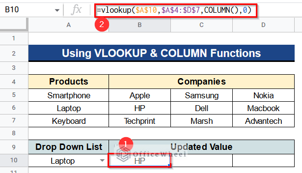
- Type the following formula in Cell B10–
=VLOOKUP($A$10,$A$4:$D$7,COLUMN(),0)- Hit Enter to get the updated value.
Formula Breakdown
- COLUMN()
It gives the column position of the desired value.
- VLOOKUP($A$10,$A$4:$D$7,COLUMN(),0)
Then it gives the search result based on Cell A10 and searches it from the range Cell A4 to D7.
- Then apply the Fill Handle tool to apply the formula in all rows.
- Finally, you’ll get the updated value in all rows.
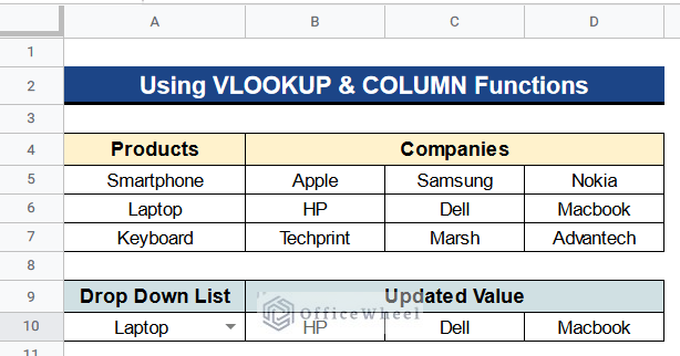
- Changing the product list from the drop down list will automatically update the corresponding cells.
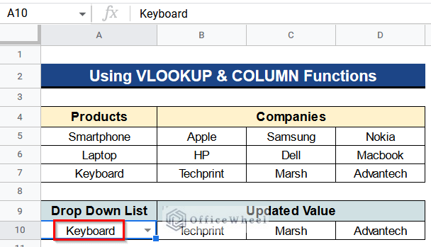
Note: You must start the dataset from the first column, Column A. otherwise the formula won’t work.
Read More: How to Use VLOOKUP with Drop Down List in Google Sheets
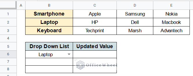
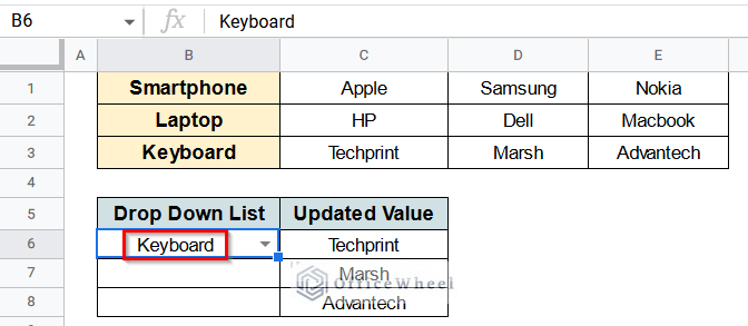
5. Merging TRANSPOSE, INDIRECT & MATCH Functions
Now we have a different situation from Method 4. We want to have the updated values in a single column based on the drop down list in Cell B6. This time we can do this by using the TRANSPOSE, INDIRECT, and MATCH functions together.
Steps:
- Generate the list in Cell B6 by applying the 3rd, 4th, and 5th steps from the first method.
- Write the following formula in Cell C6–
=TRANSPOSE(INDIRECT("C" & MATCH(B6,$B$1:$B$3,0) & ":E" & MATCH(B6,$B$1:$B$3,0)))- Press Enter to get the output.
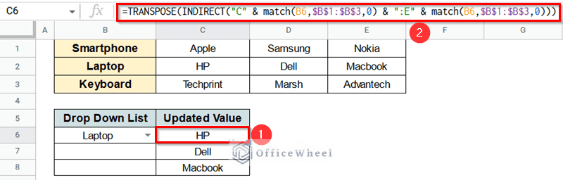
Formula Breakdown
- MATCH(B6,$B$1:$B$3,0)
This function searches for the selected product in the drop down list which is in Cell B6. Then it searches for its relative position through Cells B1 to B3.
- INDIRECT(“C” & MATCH(B6,$B$1:$B$3,0) & “:E” & MATCH(B6,$B$1:$B$3,0))
Then it gives the related value within Column C through E.
- TRANSPOSE(INDIRECT(“C” & MATCH(B6,$B$1:$B$3,0) & “:E” & MATCH(B6,$B$1:$B$3,0)))
As the values are in a row so this formula now transposes them into a column.
- If you change the product list from the drop down list, you’ll get the updated values quickly.
Note: You have to start your dataset from the first row, Row 1, otherwise the formula won’t work properly.
Read More: Multi Row Dynamic Dependent Drop Down List in Google Sheets
Conclusion
That’s all for now. Thank you for reading this article. In this article, I have tried to discuss 5 methods for updating cell values based on a selection in drop down list. If you have any queries about this article, please comment in the comment section. You will also find different articles related to google sheets on our officewheel.com. Visit the site and explore more.
Related Articles
- How to Insert a Drop-Down List in Google Sheets (2 Easy Ways)
- Create Drop Down List in Google Sheets from Another Sheet
- How to Use Data Validation in Google Sheets from Another Sheet
- Create Drop Down List for Multiple Selection in Google Sheets
- How to Remove Data Validation in Google Sheets
- Create Conditional Drop Down List in Google Sheets