Today, we will look at how to lock rows in Google Sheets in two different ways. First, the basic way with Protect Range option and the other, more sophisticated method with a criterion.
Let’s get started.
2 Ways to Lock Rows in Google Sheets
1. The Basic Way to Lock Rows in Google Sheets
The base way to lock or protect any row in Google Sheets is to do so via the Protect Range option.
In the following dataset, we have a row call Grade that contains the formula to calculate the grade obtained by each student.
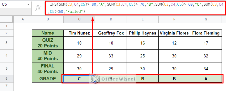
In a case like this, it is crucial that we lock this row to protect it from tampering by any other users viewing the spreadsheet.
Step 1: Select/highlight the row you want to lock. Then navigate to the Protect Range option
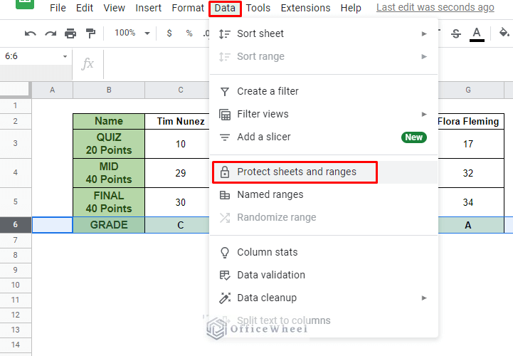
Navigating to Protect sheets and ranges from the Data tab
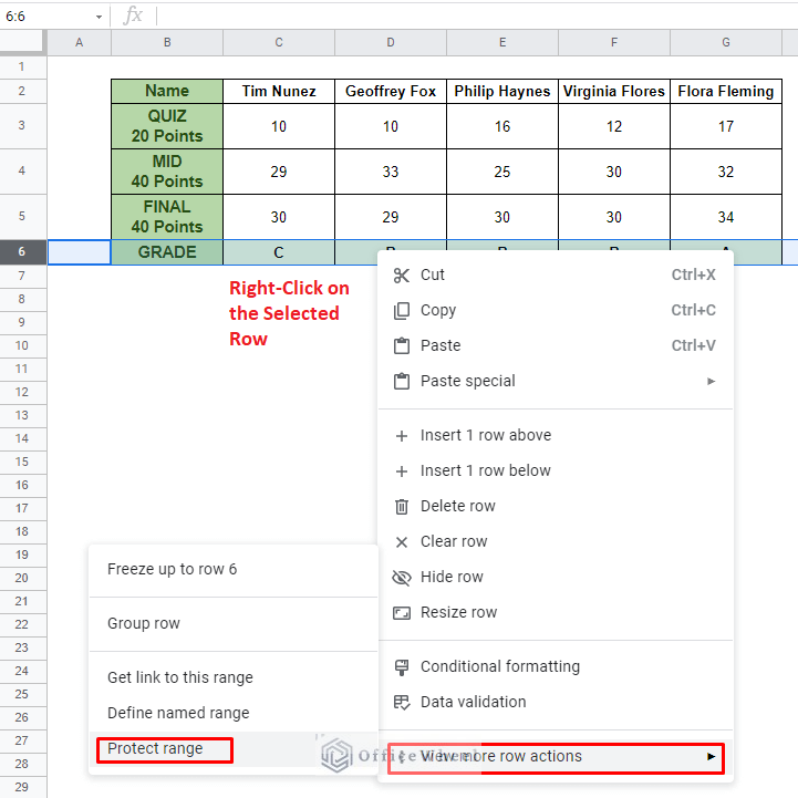
Right-clicking over the selected cells and navigating to Protect range option
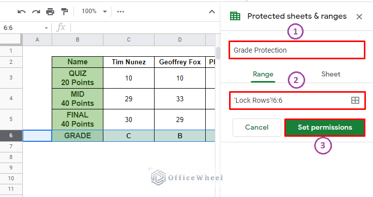
Step 2: In the Protected sheets & ranges menu, we have three preliminary sections to check.
- Name your protected range [Optional]
- Check if the locked range is correct
- Click Set permissions when you are done
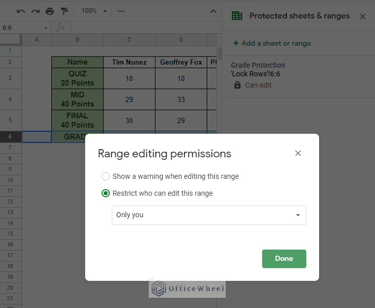
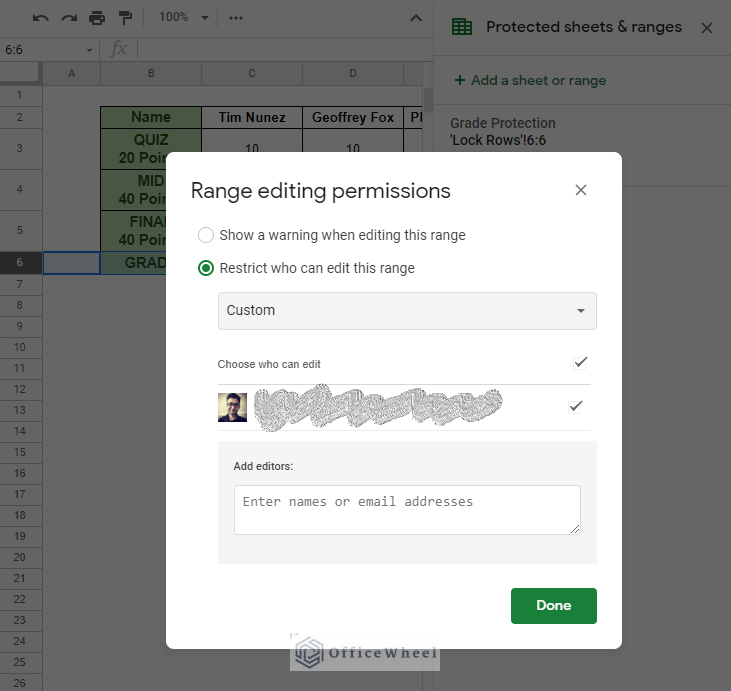
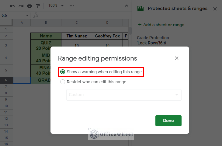
Step 3: It is in the Range editing permissions window where our locking happens. We have three options available to us depending on our needs.
- Only you: This is the option selected by default. As the name suggests, only you can make changes to the locked rows. For this example, we have chosen this option.
- Custom: Here, you can add more collaborators and permit them to edit the locked rows.
- Show a warning when editing this range: The locked rows will be free to edit, however, a warning prompt will appear when doing so.
Step 4: Click Done.
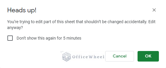
Now, if anyone other than us tries to edit the locked row, they will be hit with the following warning:
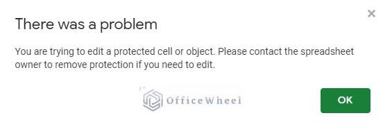
And if anyone edits after having chosen option 3, Show a warning when editing this range, from the Range editing permissions window, you will be hit with the following warning:
You can read our How to Lock Cells in Google Sheets article for an in-depth guide.
Read More: Updating Cell Values Based on Selection in Drop Down List in Google Spreadsheet
2. Conditionally Lock Rows in Google Sheets
An unorthodox, yet much needed, approach to lock rows in Google Sheets is doing so with conditions or criteria. We do this by taking advantage of the Data Validation option.
Let’s say our worksheet can be accessed by many users. But as a supervisor, I want to lock out certain rows, namely the score rows of each student. But instead of going to Protect Range to change permission every time, I want to do it with a single click.
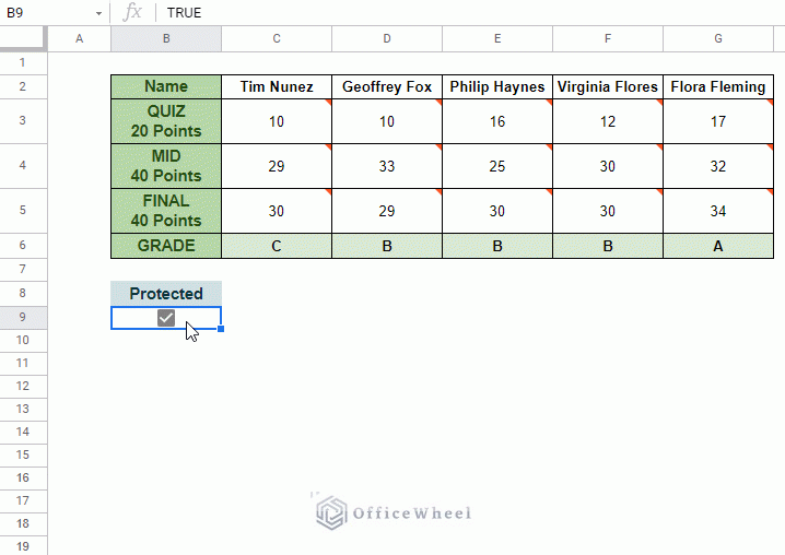
For this, we have added a checkbox to our worksheet called Protected. (Insert > Checkbox)
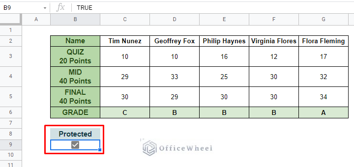
The idea is, while this checkbox is active (TRUE), no one can edit the designated rows.
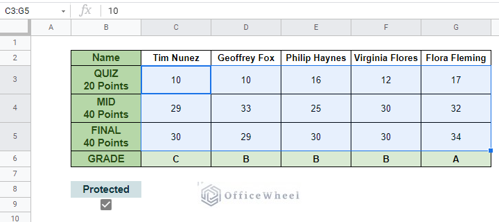
Step 1: Select the rows you want to lock. In this case, it is the Quiz, Mid, and Final rows. Cells C3:G5.
Step 2: Navigate to Data Validation from the Data tab. Data > Data validation
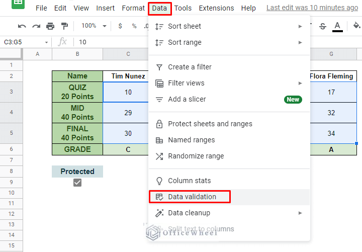
Step 3: In the Data validation window, we set three conditions.
- Select the Custom formula is option from the Criteria section.
- Set the custom formula:
=$B$9=FALSE - Check the Reject input radio button.
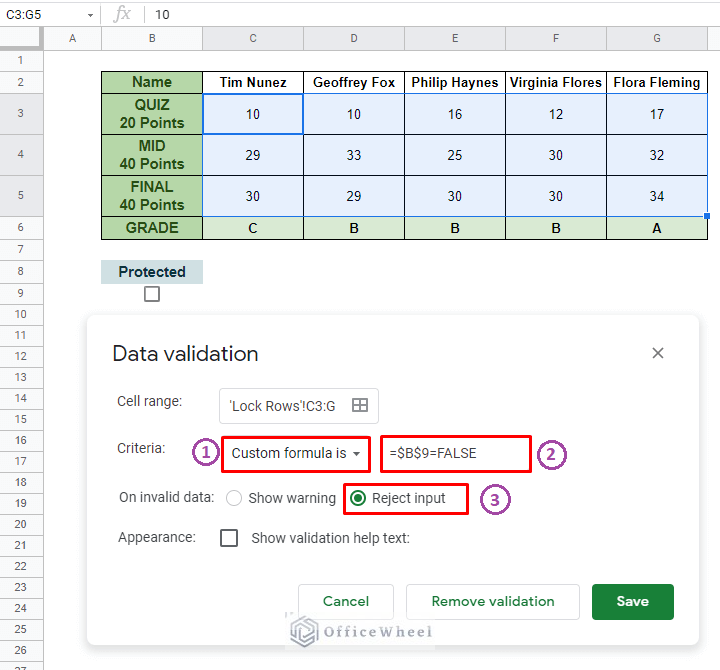
Condition Breakdown:
The Reject input option makes sure that if the custom formula condition (=$B$9=FALSE) is not true, any edits or inputs will not be accepted. In other words, the checkbox must be TRUE for the selected range of rows to be locked.
Step 4: Click Save.
Our locked rows with data validation in action:
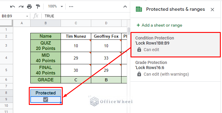
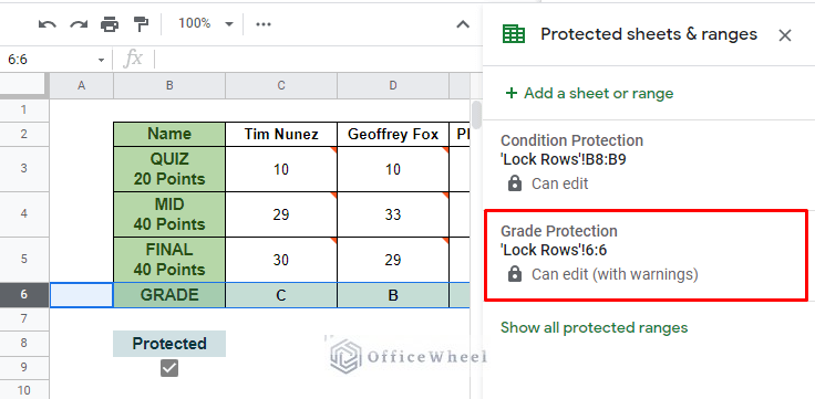
Final Protection: Locking the Conditional Cells
Locking our rows with data validation won’t mean much if anyone can flip the conditional checkbox. So we add another lock on it via the Protect Range option.
Read More: Multi Row Dynamic Dependent Drop Down List in Google Sheets
How to Unlock Rows in Google Sheets
Unlocking rows is as simple as locking them.
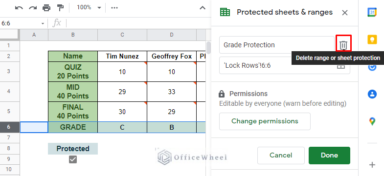
Step 1: From the Protected sheets & ranges menu select the locked range that you want to remove.
Step 2: Here, you will find a small trash can icon beside the name of the locked rows. Click on it.
Step 3: Finally, you will be prompted one last time to follow through with unlocking the rows. Click Remove.
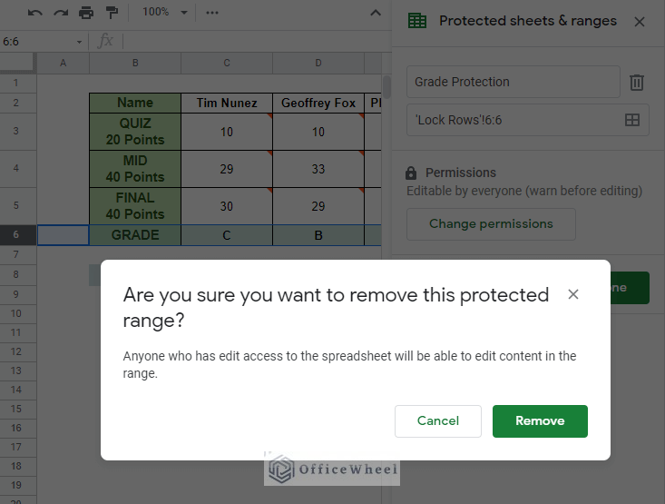
We have successfully unlocked our locked row!
Why do we need to lock cells in Google Sheets?
- You are sharing your workbook with a large audience. Many workbooks are shared publicly but leaving it on view-only mode may not cut it for every situation. You may need certain sheets or certain cells of your workbook to be restricted from third-party edits.
- You may need other users to fill up “input” cells. A form for example, where the user may need to fill up certain fields that apply to them, but not change other important cells or fields that have crucial information in them.
- Specifically, to protect cells that have complex or important formulas. The same applies to references.
Final Words
We hope that the two methods we have discussed of how to lock rows in Google Sheets come in handy for your day-to-day tasks.
However, if it is not locking/protecting rows you were looking for but freezing rows, please check out our How to Freeze Rows in Google Sheets (3 Ways) article.
Feel free to leave any queries or advice you might have for us in the comment section.
Related Articles
- How to Insert a Drop-Down List in Google Sheets (2 Easy Ways)
- Create Drop Down List in Google Sheets from Another Sheet
- How to Edit Drop-Down List in Google Sheets
- Create Drop Down List for Multiple Selection in Google Sheets
- How to Use Data Validation in Google Sheets from Another Sheet
- How to Remove Data Validation in Google Sheets