Just one thing to say, to cope with the modern world properly, we have to be fast. Spreadsheets may contain a large amount of data and we don’t have that much time to find them one by one. In this article, we will show you 4 quick easiest methods on how to use data validation and filter in Google Sheets just within a blink of an eye.
A Sample of Practice Spreadsheet
4 Easy Methods to Use Data Validation and Filter in Google Sheets
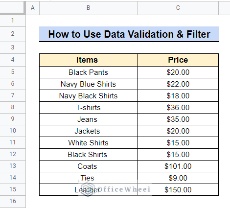
We will use the following sample dataset to describe these methods accurately. The dataset represents some cloth items’ prices.
1. Employing FILTER Function
The FILTER function looks for a particular value under a given condition and returns all information across its row or column. Here, we’ll use it to match multiple values.
Steps:
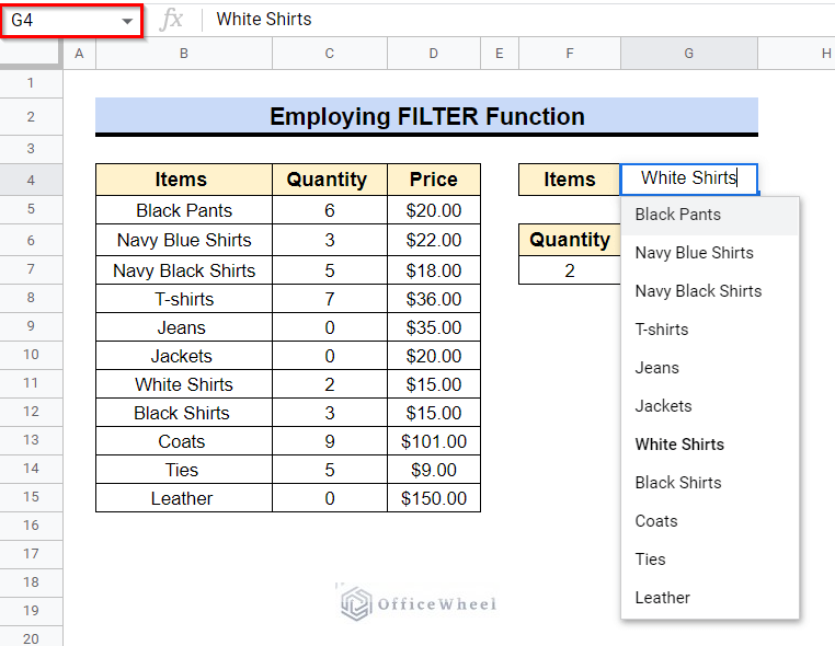
- First, in Cell G4 we will simply apply a Dropdown List for the items.
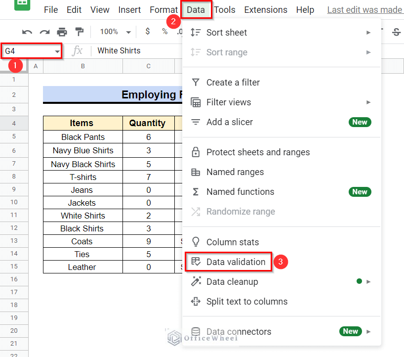
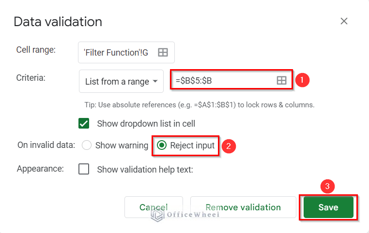
- We selected the range Cell B5 to B and locked the column and row using $. Then we select Reject input and after that click on Save.
- Now, in Cell F7 we will apply the following formula-
=FILTER(C5:D,B5:B=G5)
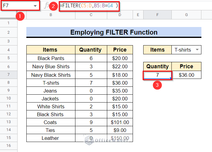
In the following formula range, Cell C5 to D indicate values we want to be appeared for what we will be searching in the filter cell. Range Cell B5 to B indicates the product name which is connected with the filter Cell G4. Now, just use the filter cell to select a product and see all the information on that.
- Select another value in Cell G4 and you will get the output according to that value.
Read More: Google Sheets: The FILTER Function (A Comprehensive Guide)
2. Applying VLOOKUP Function
The VLOOKUP function in Google Sheets performs vertical searching. This function can be used to search through a column for a specific value, and when it does, it returns a value from the same row in the specified column.
Steps:
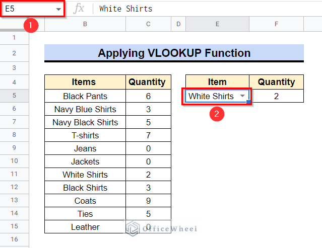
- We simply set the drop-down list in Cell E5 like previously using the Data menu in the toolbar.
- Now we will use the following formula in Cell F5–
=VLOOKUP(E5,B5:C,2,False)
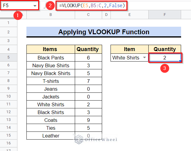
In this formula Cell E5 indicates the filter cell we have set for. Range Cell B5:C indicates the range from where it will detect the product name we gave input in filter Cell E5.
- We simply select the product from filter Cell E5 and find the availability of the product by its quantity.
Similar Readings
- How to Filter By Rows in Google Sheets (An Easy Guide)
- Filter with the AND Condition in Google Sheets (An Easy Guide)
- Filter Data Using Filter Views in Google Sheets (An Easy Guide)
3. Merging INDEX and MATCH Functions
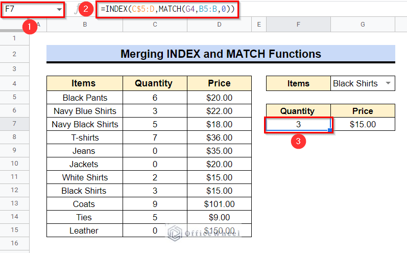
We can view a variety of data in the first argument by using the INDEX function. The row number containing the value we want to return is provided as the second argument for the MATCH function. And the combination of both is the INDEX MATCH Functions.
Steps:
- First, we will set the drop down list in Cell G4 like previously using the Data menu in the toolbar.
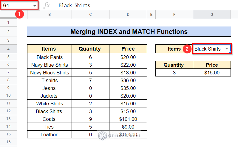
- Now in Cell F7 we will apply the following formula-
=INDEX(C$5:D,MATCH(G4,B5:B,0))
- Finally, just hit the Enter button for the output.
Formula Breakdown
- MATCH(G4,B5:B,0)
This formula finds out the cell number of the product selected in Cell G4 from the first Cell B5. Like if you select ‘Coats’ in Cell G4, it will show 9, as the product ‘Coats’ is at a distance of 9 cells from Cell B5.
- INDEX(C$5:D,MATCH(G4,B5:B,0))
By using this formula, it will show all available information of a selected product across its row.
- In the following formula Cell C$5:D indicates the ranges of values we want to get in return after selecting from Cell G4.
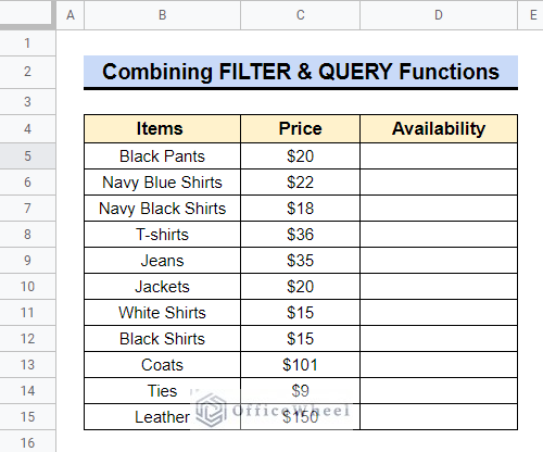
4. Combining FILTER and QUERY Functions
Presume, in the following dataset, what we want to do is to FILTER only those products that are in stock. And following the same way, we can also FILTER products out of stock. To perform this task, we’ll use the FILTER and QUERY functions.
Steps:
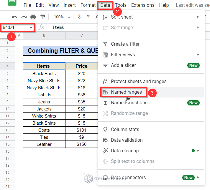
- First of all select Cell range B4:D4 and go to the Data menu in the toolbar and select Named ranges.
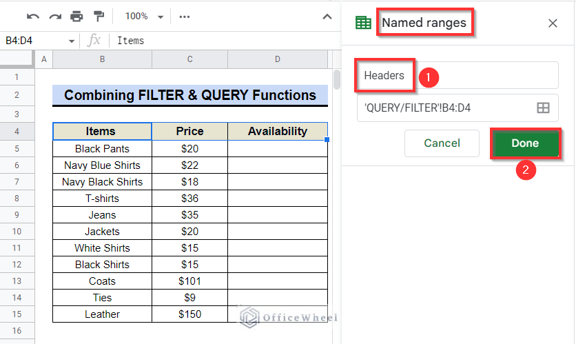
- A sidebar will appear titled Named ranges. Type “Headers” in the following empty box and then click on Done.
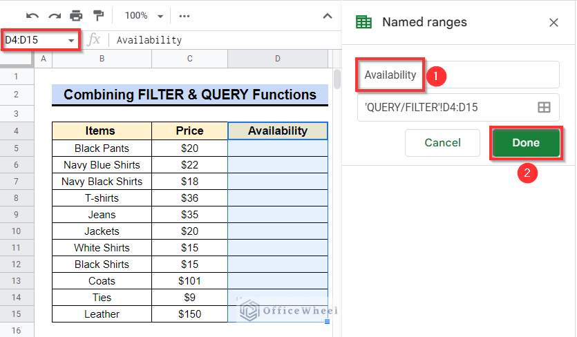
- Now, select Cell range D5:D15, and like previously go to the Data menu at the toolbar and select Named ranges, and then set the named range as “Availability” and select “Done”.
- After that, in the following dataset, select Cell F4 and apply the following formula.
=QUERY(Headers)
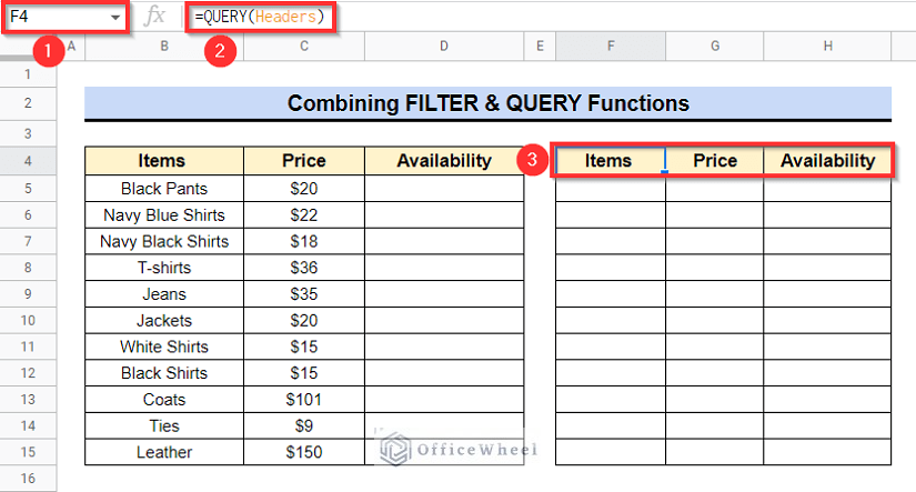
Note: The formats of Cell range F4:H4 are set as the format of Cell range B4:D4.
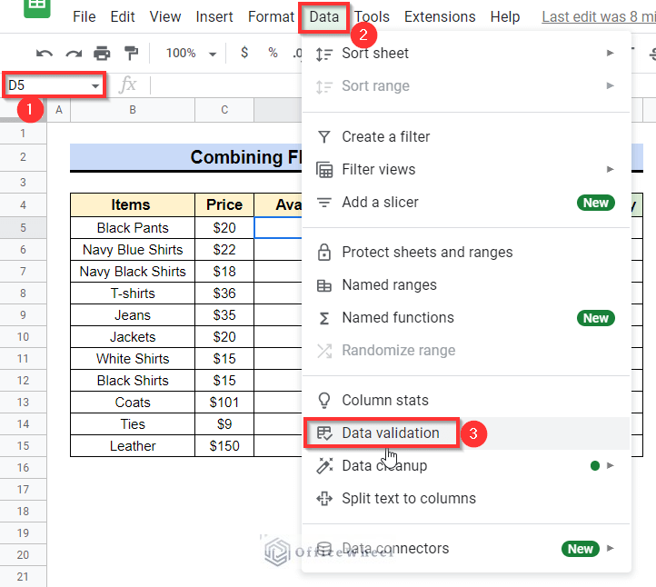
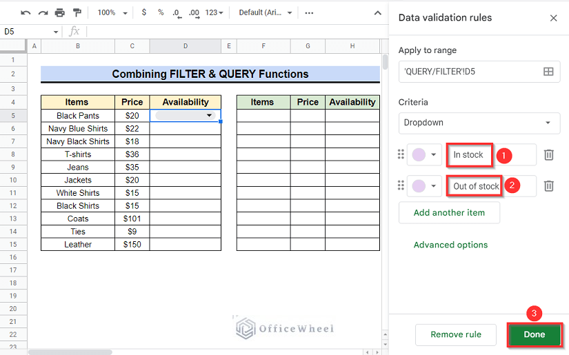
- First, we will select Cell D5 where we will set the Drop down option using Data Validation. Go to the Data option at the toolbar and click on Data validation.
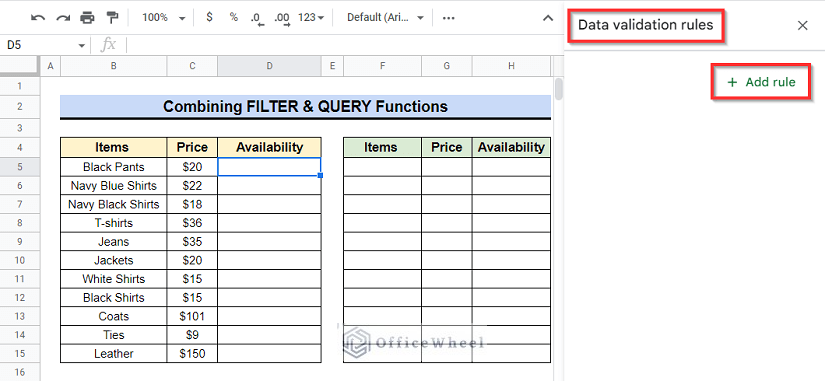
- A sidebar will appear titled “Data validation rules”. Select Add rule.
- Type “In stock” in the first box and “Out of stock” in the second one. Then click on Done.
- Now using the Fill Handle icon as shown in the circled portion simply Drag down.
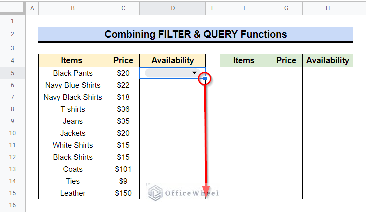
- This will apply the Dropdown option for the rest of the cells as well.
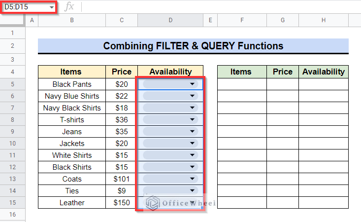
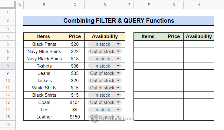
- Now, set the availability of the products using those dropdown options. Suppose, the availability of all the following products is as follows.
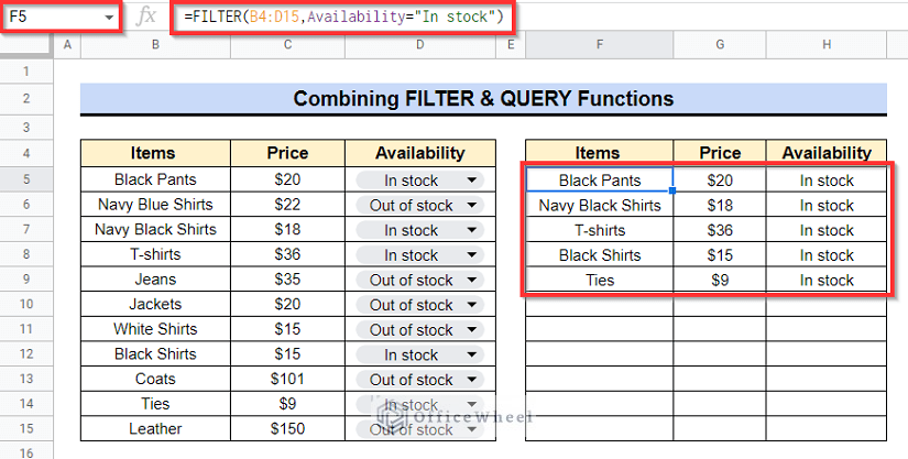
- As mentioned before, what we want to do is FILTER only those products that are in stock. Activate Cell F5 and apply the following formula.
=FILTER(B4:D15,Availability="In stock")
The formula here will look for the corresponding values for Availability=”In stock” command.
We will get the output as follows.
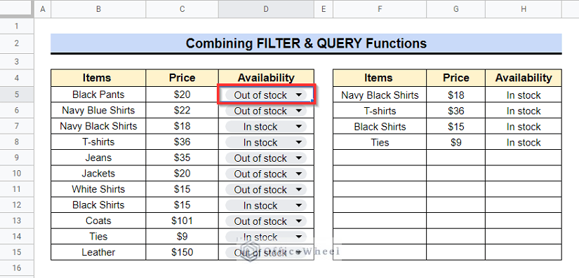
- Now, suppose I set the availability of the product “Black Pants” as “Out of stock”, it will not appear in the result section.
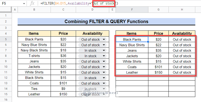
- If you want to know which products are out of stock, simply type “Out of stock” in the formula and press Enter-
=FILTER(B4:D15,Availability="Out of stock")
And we will get to know about products that are out of stock.
Read More: How to Filter with QUERY for Multiple Criteria in Google Sheets (An Easy Guide)
Conclusion
These 4 methods of using the data validation and filter in Google Sheets will give you instantaneous speed. I hope this will work for you the way you wanted. Visit officewheel.com to explore more.
Related Articles
- How to Find and Replace Blank Cells in Google Sheets
- Use Wildcard in Google Sheets (3 Practical Examples)
- How to Filter for Multiple Conditions in Google Sheets (2 Easy Ways)
- Filter Entries if it Does Not Contain Value in Google Sheets (2 Easy Ways)
- How to Filter Based on a Cell Value in Google Sheets (2 Easy ways)
- Applying Filter with REGEXMATCH Function in Google Sheets (Easy Examples
- How to Filter Custom Formula in Google Sheets (3 Easy Examples)
- How to Create Filter Views in Google Sheets (An Easy Guide)