How to Filter By Rows in Google Sheets (An Easy Guide)

Typically, datasets are presented vertically, with column headers followed by a vertical list of data. But sometimes, you may have data that is given horizontally like this:

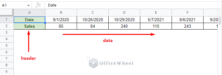
Unless you want to change the orientation, you have to filter this data horizontally.

That said, in this article, we will look at how to filter data by rows in Google Sheets. And it is simple to do so.

Let’s get started.

How to Filter by Rows (Filter Horizontally) in Google Sheets

It is important to note that the only way to filter by rows in Google Sheets is by using the FILTER function. There is still no way to make the default filter feature recognize if the data is presented horizontally or not.

The FILTER function syntax:

This function is perfect since it allows users to define the data range for both the source data and the filter condition.

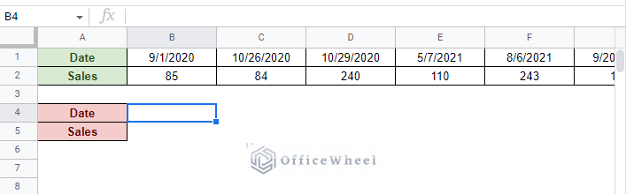
To show how it works, let’s consider a simple example dataset. Here we will try to filter all entries that have a Sales value of less than 100.

Step 1: Open the FILTER function and select the first cell of the data. For us, it is cell B1.

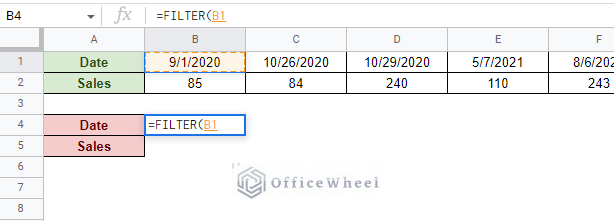
This represents the beginning of the data range.

Step 2: You can simply SHIFT+Click the last cell of the dataset to complete the data range, or you can make the formula more dynamic by typing the row number. So, the data range will be:

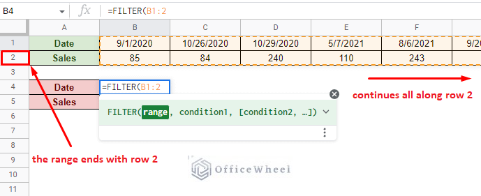
This is how the user can define that the data range is horizontal, and not the typical vertical arrangement. This also determines how the filtered result will be presented.

Step 3: As for the condition, we will follow the same syntax for the range. Since the filter condition is “less than 100 Sales”, the condition will be:

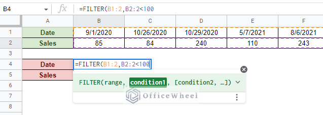
Step 4: Close parentheses and press ENTER.

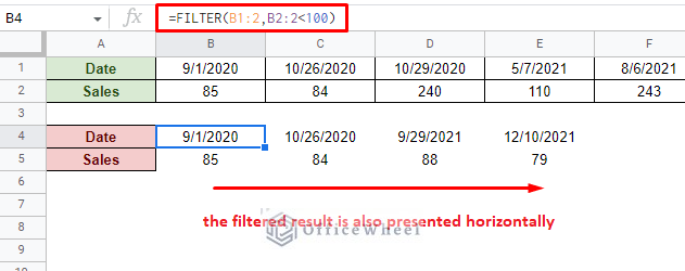
Known Issues with Mismatched Data Ranges

Since filtering by rows is an uncommon process, new users may face some errors when handling horizontal data with the FILTER function. Specifically, in regards to how the data range works in the FILTER function.

For example, you can see in the following image that we have set the range for the condition to B2:K2, with K2 being the last cell of the dataset.

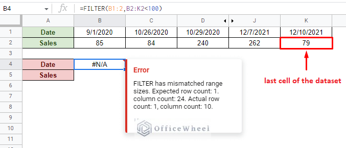
However, this range for the condition does not match the number of columns that was input for the data range of the FILTER function, B1:2, where the 2 represent the entirety of row 2.

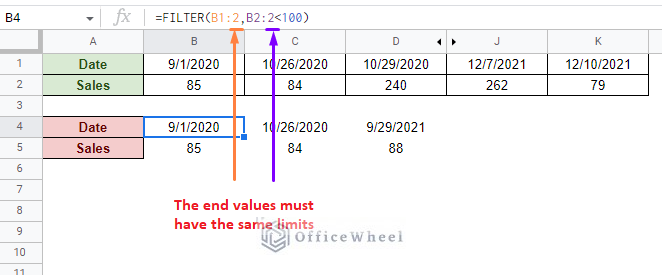
So, it is crucial to make sure that the range of the values of the condition has the same limits as the data range.

In other words, the end value of both the data range and condition range must have the same limits:

Filter for Multiple Conditions Horizontally in Google Sheets

Filtering for multiple conditions is common in Google Sheets. Let’s see how we can do so for horizontally arranged data.

From the following dataset, let’s try to filter entries that have over 200 Sales in the North Region:

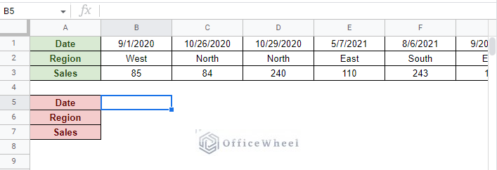
As you can see, we’ve added a new row of values to the source data, Region. This will help us to show that the FILTER function works as usual with both text and numerical values, even if they are horizontally aligned.

Step 1: Open the filter function and input the data range.

Step 2: Input the first condition. We are looking for the text “North” in the Region row.

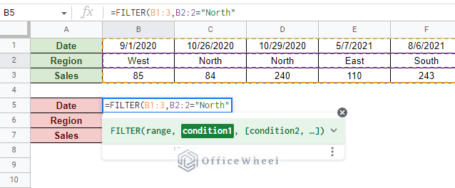
Step 3: Input the second condition. We want Sales that have a value greater than 200.

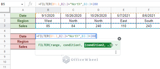
Step 4: Close parentheses and press ENTER to see the results.

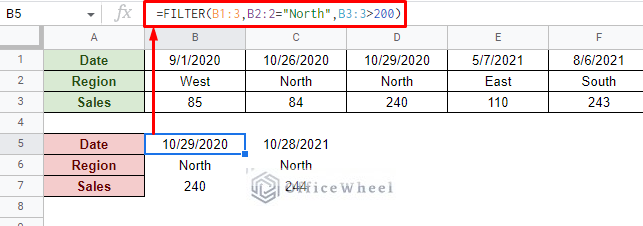
We get only two entries that satisfy both of the conditions. Notice also that regardless of the number of rows in the source dataset, as long as it is in the data range, we will get all the values necessary.

Alternatively, if we want to filter for either of the conditions, filter with the OR condition, in other words, we can apply the following formula:

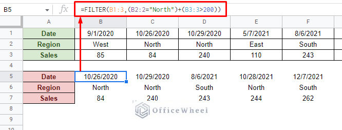
Read More: Filter Values that Contains Multiple Text Criteria in Google Sheets (2 Easy Ways)

Final Words

That concludes all the ways we can use to filter by rows in Google Sheets. While we cannot use the default filter feature to do so, the FILTER function steps up quite nicely to the occasion as long as the data range for both the source data and conditions is correct.

Feel free to leave any queries or advice you may have in the comments section below.

Related Articles for Reading:

• How to Find and Replace Blank Cells in Google Sheets
• How to Use Wildcard in Google Sheets (3 Practical Examples)
• How to Use Data Validation and Filter in Google Sheets (4 Ways)
• Applying Filter with REGEXMATCH Function in Google Sheets (Easy Examples)
• Google Sheets: Filter Data if it Contains Value (A Comprehensive Guide)
• Google Sheets: Filter for Multiple Criteria with Formula (2 Easy Ways)
• How to Filter by Condition Using a Custom Formula in Google Sheets (3 Easy Examples)
• Filter Entries if it Does Not Contain Value in Google Sheets (2 Easy Ways)