How to Add Color to Drop Down List in Google Sheets (Easy Steps)

This article highlights how to add color to the drop down list in Google Sheets. Using a drop down list is very useful to choose a specific option from multiple options. Adding color to the drop down list makes it easier to differentiate between them. Follow the article to learn how to do that in a few easy steps.

Table of Contents

Step by Step Procedure to Add Color to Dropdown List in Google Sheets

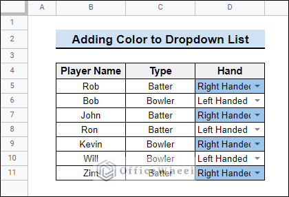
Consider the following picture showing a dropdown list with colors. The dropdown list is added to select if a player is Right Handed or Left Handed. But the colors added to the dropdown list made it much easier to know the difference.

Follow the steps below to learn how to add color to the drop down list in Google Sheets as shown above.

Step 1: Select the Range

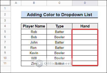
First, select the range where you need to create the dropdown list. In this case, the cell range is D5:D11.

Step 2: Apply Data Validation

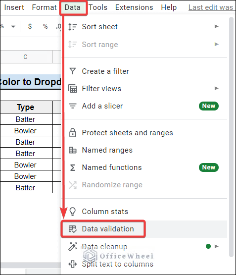
Then go to Data >> Data Validation as shown in the picture below.

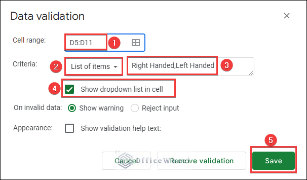
Next, the Data Validation dialogue box will appear. In the dialogue box, you will see the cell range selected earlier. Change it if needed.
After that select List of items as Criteria. You can also choose other criteria using the dropdown list there. Then write the options that you need to add to the dropdown list and separate them with commas.
Next, check the Show dropdown list in cell checkbox and click on Save.

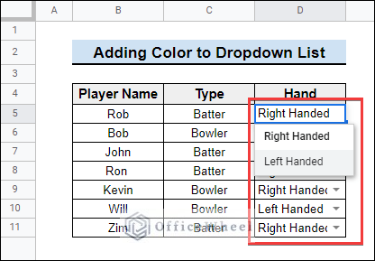
After that, the dropdown list will be created as follows.

Step 3: Use Conditional Formatting

In the final step, you need to apply Conditional Formatting to change the color of the dropdown list.

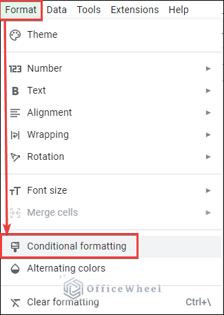
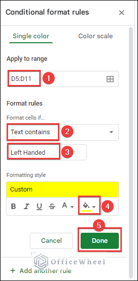
First, select the range D5:D11 and go to Format>>Conditional Formatting. Then the dialog box for Conditional Format rules will appear.

Here the range is previously selected. Now you can choose any formula as required from the Format Rules.

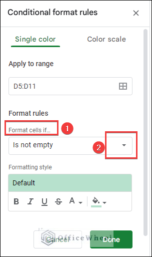
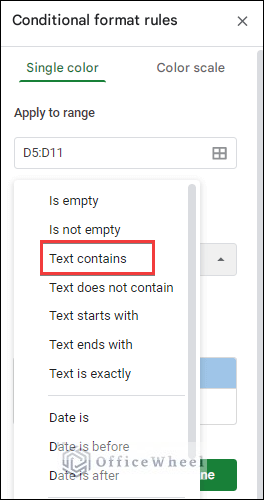
In this case, choose Text contains from Format cells if option.

Type the first option of the dropdown list i.e Right Handed in the Value or Formula box below.

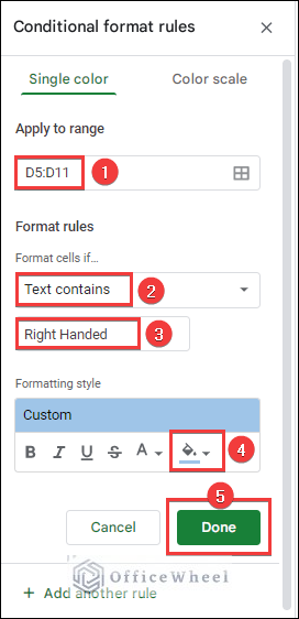
Then, select a color using the Fill Color option from the Formatting Style. This will add color to the first option of your dropdown list.

Now add color to the Left Handed option by clicking Add another rule.

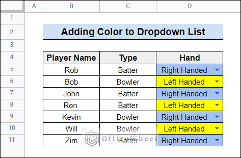
Finally, you will get the following result.

Things to Remember

Make sure you have selected the correct range before applying Data Validation.
You can also add color to a drop-down list in a single cell and drag it to copy as required.

Conclusion

Now you know how to add color to the drop down list in Google Sheets. Please use the comment section below for further queries or suggestions. Hopefully, it will help you to visualize your data more properly. You may also visit our OfficeWheel blog to explore more about Google Sheets.