We are pretty familiar to transpose multiple rows into columns, but transposing to one column is a bit different and difficult. We will show 3 easy methods to transpose multiple rows into one column using FLATTEN, INDEX, TRANSPOSE, and other functions in Google Sheets with clear images and steps.
A Sample of Practice Spreadsheet
You can download Google Sheets from here and practice very quickly.
3 Quick Tricks to Transpose Multiple Rows into One Column in Google Sheets
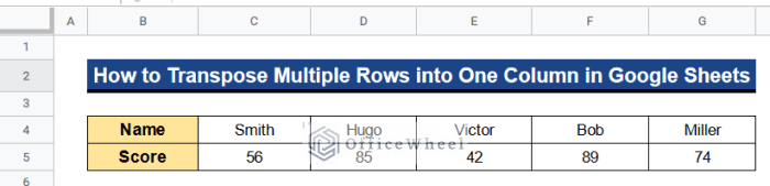
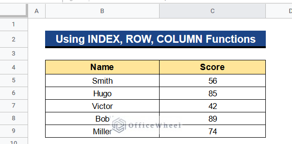
First, let’s get introduced to our dataset. Here we can see the names and scores of some people. Now we will transpose multiple rows into one column by using different functions.
1. Apply FLATTEN Function in Google Sheets to Transpose Multiple Rows into One Column
The first method uses the FLATTEN function to transpose two rows into one single column. This method is very easy because it uses only a simple function.
Steps:
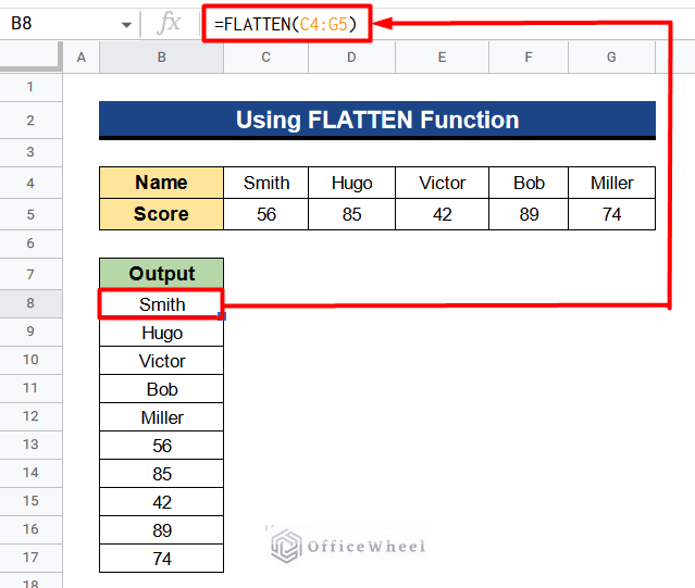
- Type the following formula in Cell B8–
=FLATTEN(C4:G5)- Hit Enter button to get the output into a single column.
2. Transpose Multiple Rows into One Column Using Combination of INDEX, INT, ROW, COLUMNS, and MOD Functions
In this second method, we will use a combination of different functions named INDEX, INT, ROW, COLUMNS, and MOD Functions. This method is lengthy because of using so many functions but is useful in some particular cases.
Steps:
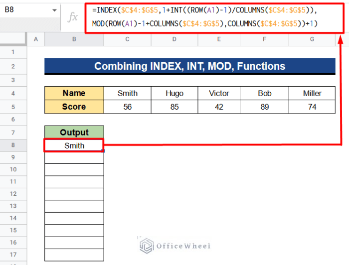
- Write the following formula in Cell B8–
= INDEX($C$4:$G$5,1+INT((ROW(A1)-1)/COLUMNS($C$4:$G$5)),MOD(ROW(A1)-1+ COLUMNS($C$4:$G$5),COLUMNS($C$4:$G$5))+1)- Press Enter to get the result.
Formula Breakdown:
- COLUMNS($C$4:$G$5), COLUMNS($C$4:$G$5), COLUMNS($C$4:$G$5)
Firstly, it gives the no of columns in the dataset. Here in our dataset, there are total 5 columns and this formula includes them in the calculation process.
- ROW(A1)
Secondly, it gives the row number of Cell A1 in our dataset.
- MOD(ROW(A1)-1+COLUMNS($C$4:$G$5),COLUMNS($C$4:$G$5))
Afterward, the above formula calculates the 5 columns and 2 rows of our dataset.
- INT((ROW(A1)-1)/COLUMNS($C$4:$G$5)),MOD(ROW(A1)-1+COLUMNS($C$4:$G$5), COLUMNS($C$4:$G$5))
Then this formula gives the nearest integer value of the numbers present in our sheets.
- INDEX($C$4:$G$5,1+INT((ROW(A1)-1)/COLUMNS($C$4:$G$5)),MOD(ROW(A1)-1+COLUMNS($C$4:$G$5),COLUMNS($C$4:$G$5))+1)
Finally, the INDEX function will return the first value and put that in Cell B8.
- Then apply the Fill Handle tool to use the formula in all columns.
![]()
- You will get the following output.
![]()
3. Combine TRANSPOSE, SPLIT, TEXTJOIN, FILTER, ISEVEN, ISODD, and ROW Functions to Get Results in Single Column
Sometimes we need results for only even rows or odd rows, not all rows. Then we can apply this method. In this method, we will assign the combination of TRANSPOSE, SPLIT, TEXTJOIN, FILTER, ISEVEN, ISODD, and ROW functions to obtain results. The only difference is that we will use the ISEVEN function to get output for even rows and the ISODD function for odd rows. So we’ll have to apply the formula two times.
Steps:
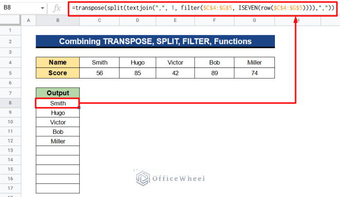
- Type the following formula in Cell B8–
=TRANSPOSE(SPLIT(TEXTJOIN(",", 1, FILTER($C$4:$G$5, ISEVEN(ROW($C$4:$G$5)))),","))- Push Enter button to get the result for even rows.
- Again, type the following formula in Cell B13–
=TRANSPOSE(SPLIT(TEXTJOIN(",", 1, FILTER($C$4:$G$5, ISEVEN(ROW($C$4:$G$5)))),","))- Hit Enter button to get the result for odd rows.
![]()
Formula Breakdown:
- ISEVEN(ROW($C$4:$G$5))
At first, this formula collects the information from even rows. Like in this case we have Names in Row 4 which is even.
- ISODD(ROW($C$4:$G$5))
This formula works like the above-mentioned formula instead it works for odd rows. We have Score in Row 5 which is odd.
- FILTER($C$4:$G$5, ISEVEN(ROW($C$4:$G$5)))
Then this formula filters out the even or odd rows based on given conditions. Here it will only filter the even row which is Row 4.
- TEXTJOIN(“,”, 1, FILTER($C$4:$G$5, ISEVEN(ROW($C$4:$G$5))))
Next, this formula will join the values of the specified rows likewise here is Row 4.
- SPLIT(TEXTJOIN(“,”, 1, FILTER($C$4:$G$5, ISEVEN(ROW($C$4:$G$5)))),”,”)
Afterward, the above formula will divide each joining text of Row 4 to put them into separate cells of one single column, Column B.
- TRANSPOSE(SPLIT(TEXTJOIN(“,”, 1, FILTER($C$4:$G$5, ISEVEN(ROW($C$4:$G$5)))),”,”))
Finally, it transposes the given rows, Row 4 and Row 5 into one single column, Column B.
How to Transpose Every n Row in Google Sheets
Now we will look into a different case where we need results for every n row in Google Sheets. We will apply a combination of INDEX, ROW, and COLUMN functions to get the desired output.
Here is our dataset where we have names in Column B and scores in Column C. We want to get the names in Column B of every 2nd row.
Steps:
- Write the following formula in Cell B12–
=INDEX($B$4:$B$9,ROW(B1)*2-2+COLUMN(B1))- Press Enter to get the result.
![]()
Formula Breakdown:
- ROW(B1)
Firstly the formula gives the row number of Cell B1.
- COLUMN(B1)
Secondly, it offers the column number of Cell B1.
- INDEX($B$4:$B$9,ROW(B1)*2-2+COLUMN(B1))
Finally, the above formula shows the desired value of every 2nd row of Column B.
- Then apply the Fill Handle tool to apply the formula in all columns.
![]()
- You will get the following result. Moreover, you will see that we get the names from every 2nd row of Column B.
![]()
How to Transpose Row to Column in Google Sheets
We can also transpose row to column in google sheets very quickly by Paste Special menu and TRANSPOSE function. This method is useful when we have to get the output quickly and we do not need results in just one column.
1. Use Paste Special
Paste special is a very distinguished feature in Google Sheets. We can easily transpose any row to column or vice versa by this method.
Steps:
- Select all the cells you want to copy and press Ctrl+C.
- Right-click on the selected cells and go to the Paste special menu and select Transposed.
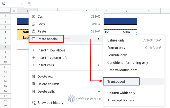
- You will get the following result.
![]()
Read More: How to Transpose Columns to Rows in Google Sheets (3 Methods)
2. Apply the TRANSPOSE Function
We can also use the TRANSPOSE function to transpose any row to column. This function is very easy to remember.
Steps:
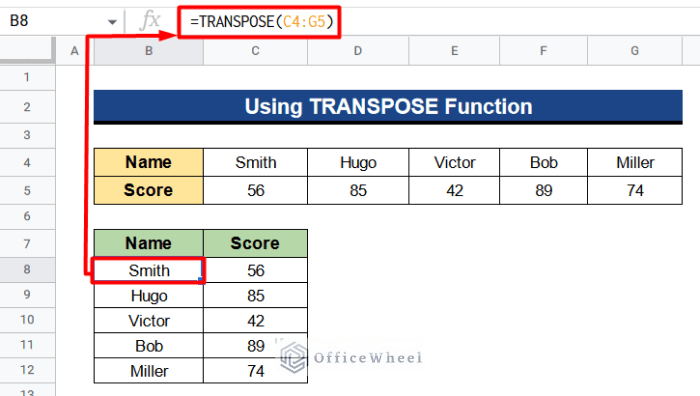
- Type the following formula in Cell B8–
=TRANSPOSE(C4:G5)- Push Enter button to get the result.
Read More: Change Columns to Rows in Google Sheets (3 Easy Ways)
What to Do When Paste Transpose Is Not Working in Google Sheets
TRANSPOSE function does not work when there is no space where the value would take place. Like in the following case we have a value in Cell B11.
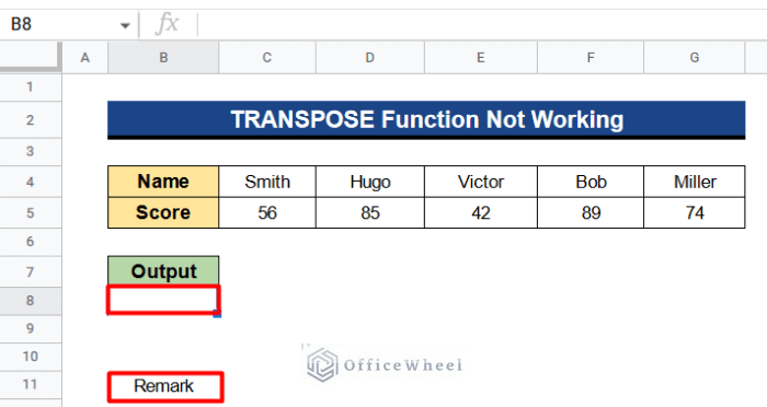
Applying the TRANSPOSE function in Cell B8 gives an error message. From the message we can see that it is telling us, we have a value in Cell B11.
![]()
When we remove the value from Cell B11 then the TRANSPOSE function will work smoothly.
Read More: [Solved!] Paste Transpose Is Not Working in Google Sheets
Conclusion
That’s all for now. Thank you for reading this article. In this article, I try to discuss different ways of transposing in Google sheets but emphasize transposing multiple rows into a single column. If you have any queries please leave a comment in the comment section. You will also find different articles related to google sheets on our officewheel.com. Visit the site and explore more.