A dependent drop down list is used when one wants to show only relevant information for subsequent drop downs. While there are a few helpful ways of creating a dependent drop down list for a single cell in Google Sheets, creating dependent drop down lists for an entire column has some complexities. Here, in this article, we have shown 2 practical ways of creating a dependent drop down list in Google Sheets to minimize those complexities.
2 Practical Methods to Create Dependent Drop Down List for Entire Column
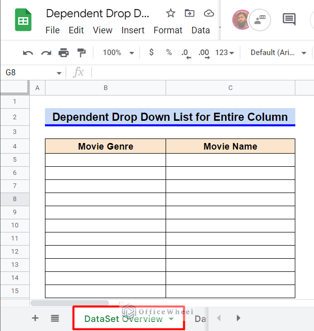
First, let’s know about our dataset. We need two worksheets named “DataSet Overview” and “DataSet Options” respectively. The first worksheet has two columns where we will create a dependent drop down list for movie genres and movie names. The user can select a movie genre in the first column and a subsequent movie name in the second column for as many rows as he/she likes (for example, selecting a movie night schedule for a year). However, we have taken only 11 rows only.
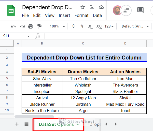
In the second worksheet, we have some famous movie names classified according to their genre. I have taken 3 movie genres and 6 movies for each of the genres.
1. Using Formula in Google Sheets
One can use Data Validation and then combine a few functions like TRANSPOSE, INDEX, and MATCH in a formula to create a dependent drop down list for an entire column in Google Sheets. Here, we require two worksheets for this method.
Step 1: Create the First Drop Down List
Firstly, let’s create our first dependent drop down list.
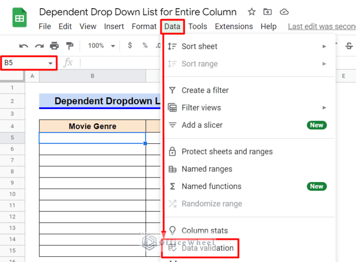
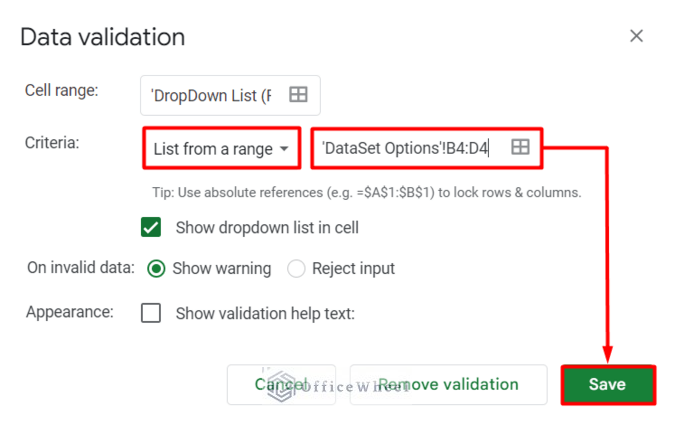
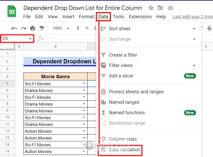
- Select Cell B5 from the worksheet “DropDown List (Formula)” and then go to the Data ribbon and click on Data Validation.
- In the popped-out window, set List from a range as ‘DataSet Options’!B4:D4 and then click on Save. Note that, we haven’t fixed the cells B4:D4 using the $ sign. But Google Sheets assumes fixed cells in Data Validation by default. This will create some problems in section 1.3.
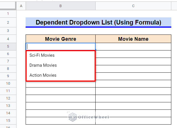
- The first drop down list has now been created in Cell B5. Click on the drop down icon to see the list.
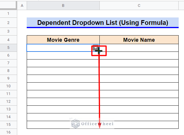
- Now again select Cell B5 and use the Fill Handle icon to copy the formula into other cells of the icon.
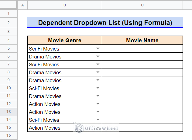
- Since Google Sheets fixes the cells by default in Data Validation, we will get the same list in every cell of Column B. Select any value from each of the cells.
Read More: Create Drop Down List in Google Sheets from Another Sheet
Step 2: Apply Formula to Create Range for Second Drop Down List
In this section, we will combine TRANSPOSE, INDEX, and MATCH functions in a formula to create process data in the “Helper” worksheet for our second drop down list.
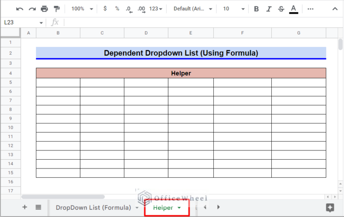
- Take a worksheet like the following and name it “Helper”.
- In the “Helper” worksheet, select Cell B5 and type the following formula:
TRANSPOSE(INDEX('DataSet Options'!$B$5:$D$10,,MATCH('DropDown List (Formula)'!B5,'DataSet Options'!$B$4:$D$4,0)))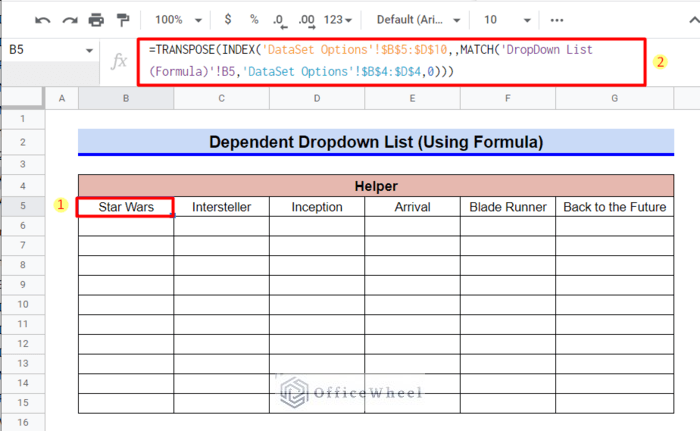
Formula Breakdown:
- MATCH(‘DropDown List (Formula)’!B5,’DataSet Options’!$B$4:$D$4,0)
The MATCH function returns the relative position of the data in Cell B5 of the worksheet “DropDown List (Formula)” in the array B4:D4 of worksheet “DataSet Options” if an exact match occurs.
- INDEX(‘DataSet Options’!$B$5:$D$10,,MATCH(‘DropDown List (Formula)’!B5,’DataSet Options’!$B$4:$D$4,0))
The INDEX function returns all the rows in the column specified by the MATCH function.
- TRANSPOSE(INDEX(‘DataSet Options’!$B$5:$D$10,,MATCH(‘DropDown List (Formula)’!B5,’DataSet Options’!$B$4:$D$4,0)))
The TRANSPOSE function converts the column returned by the INDEX function into a row.
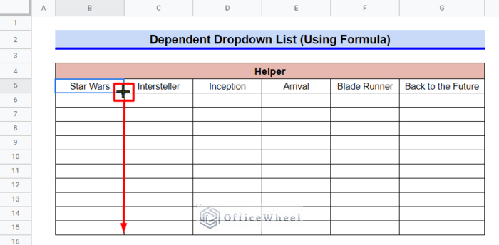
- Select Cell B5 again and use the Fill Handle to copy the formula in other cells of the column.
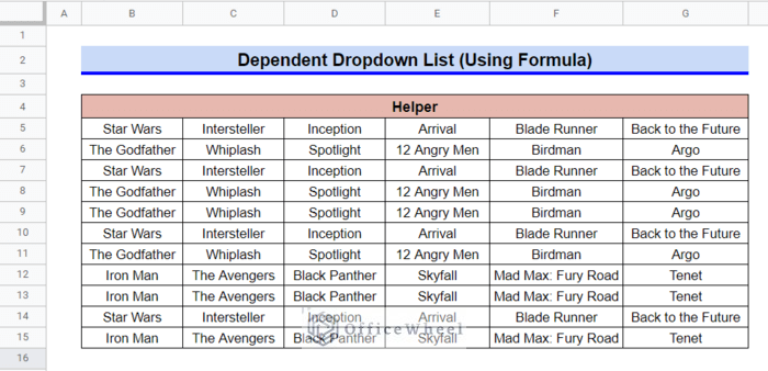
- Processed data for the second drop down list is now ready.
Read More: How to Edit Drop-Down List in Google Sheets
Similar Readings
- How to Use Data Validation in Google Sheets from Another Sheet
- Multi Row Dynamic Dependent Drop Down List in Google Sheets
- How To Lock Rows In Google Sheets (2 Easy Ways)
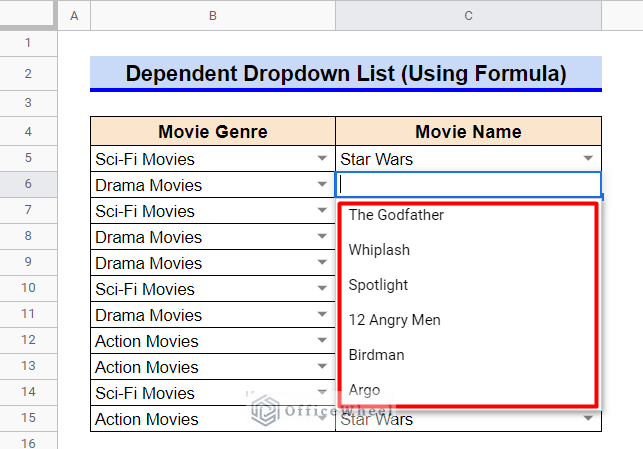
Step 3: Create the Second Drop Down List
Finally, we create our second drop down list.
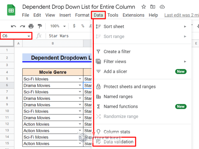
- Return to the “DropDown List (Formula)” worksheet and select Cell C5. Go to the Data ribbon and click on Data Validation.
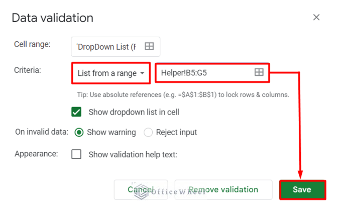
- In the popped-out window, set List from a range as Helper!B4:G5 and then click on Save.
- A dependent drop down list has now been created at Cell C5. Click on the drop down icon to see the list. Select any movie from the list.
11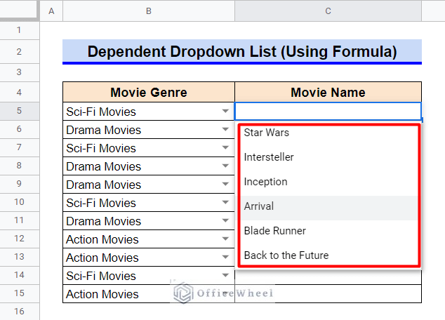
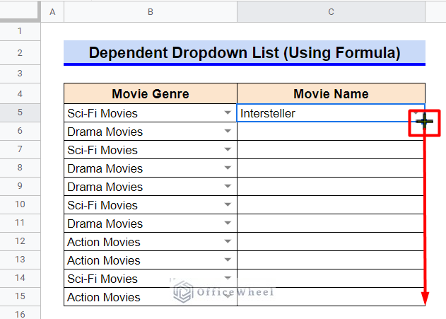
- Select Cell C5 and use the Fill Handle to copy the formula in other cells of Column C.
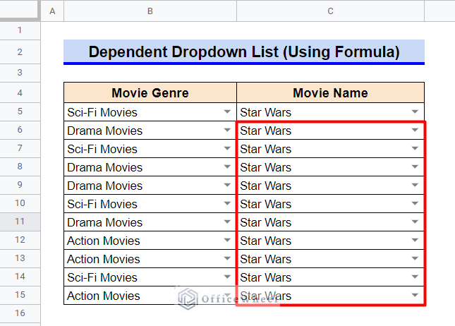
- Here, the same formula has been copied in every cell. It is because Google Sheets fixes the values in Data Validation by default.
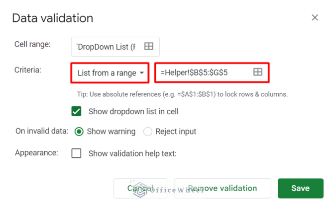
- The List from a range is set as Helper!$B$5:$G$5 which is the validation for Cell C5.
- Change the List from a range to Helper!$B$6:$G$6 click on Save.
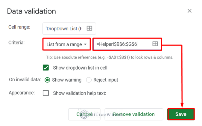
- The correct drop down has now been created in Cell C6.
- Manually change the List from a range for other cells of Column C by following the previous four steps. Now, finally have our dependent drop down list for the entire column.
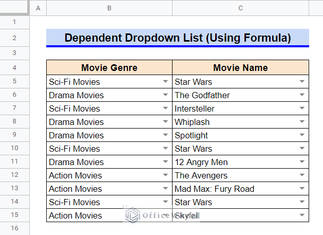
The manual change of the List from a range makes this method inefficient for large data. You can use the second method for large data.
Read More: Create Multiple Dependent Drop Down List in Google Sheets
2. Using Apps Script
To avoid manual operations, we will use Apps Script for data validation in the second dropdown list.
Steps:
- Follow the first five steps from Section 1.1 to create the first drop down list in cells of Column B.
- Now, go to the Extensions ribbon and click on Apps Script.
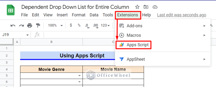
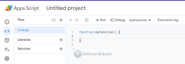
- A new window like the following will open in the browser.
- Rename the project according to your need. We have named it “DropDown List for Entire Column”.
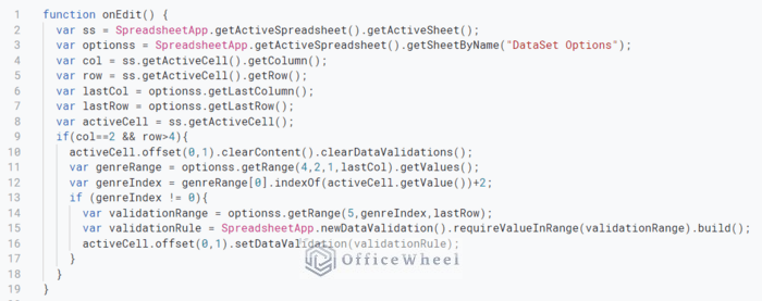
- Now, enter the following script:
function onEdit() {
  var ss = SpreadsheetApp.getActiveSpreadsheet().getActiveSheet();
  var optionss = SpreadsheetApp.getActiveSpreadsheet().getSheetByName("DataSet Options");
  var col = ss.getActiveCell().getColumn();
  var row = ss.getActiveCell().getRow();
  var lastCol = optionss.getLastColumn();
  var lastRow = optionss.getLastRow();
  var activeCell = ss.getActiveCell();
  if(col==2 && row>4){
    activeCell.offset(0,1).clearContent().clearDataValidations();
    var genreRange = optionss.getRange(4,2,1,lastCol).getValues();
    var genreIndex = genreRange[0].indexOf(activeCell.getValue())+2;
    if (genreIndex != 0){
      var validationRange = optionss.getRange(5,genreIndex,lastRow);
      var validationRule = SpreadsheetApp.newDataValidation().requireValueInRange(validationRange).build();
      activeCell.offset(0,1).setDataValidation(validationRule);
    }
  }
}
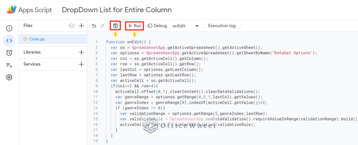
- After completing the script, first, click on Save project and then click on Run to apply the script.
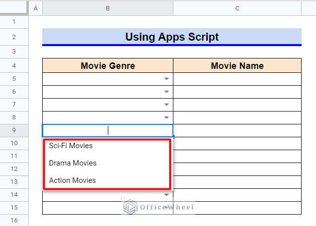
- Return to the worksheet and click on the drop down icons in cells of Column B. Choose any movie genre for each of the cells.
- After choosing a movie genre in cells of Column B, drop down icons will appear in subsequent cells of Column C.
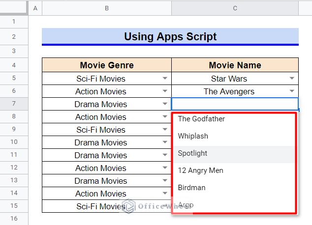
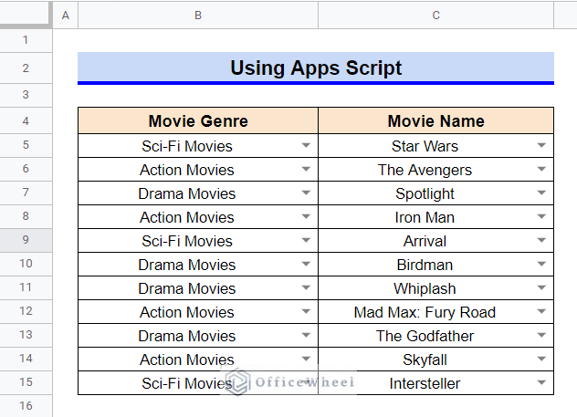
- The second drop down list is now complete and you can choose any movie name from the list for each cell of Column C.
Things to Be Considered
- Google Sheets fixes the cells by default in List from a range during Data Validation.
- Inserting worksheet names correctly in Apps Script is mandatory for correct output.
- Use meaningful variable names in Apps Script.
Conclusion
This concludes our article on how to create a dependent drop down list for an entire column in Google Sheets. We hope the mentioned methods fulfill your requirements. Feel free to leave any queries or advice in the comment section.
Related Articles
- How to Create Dependent Drop Down List in Google Sheets
- Add Color to Drop Down List in Google Sheets (Easy Steps)
- How to Use VLOOKUP with Drop Down List in Google Sheets
- Create Conditional Drop Down List in Google Sheets
- How to Remove Data Validation in Google Sheets
- Updating Cell Values Based on Selection in Drop Down List in Google Spreadsheet