How to Use VLOOKUP Function with Wildcard in Google Sheets

We use the VLOOKUP function to look up any value in a given data range. In addition to that, we can add Wildcard into the VLOOKUP formula to search for any value with a partial match. In the following article, I’ll show 2 suitable examples to use the VLOOKUP function with Wildcard in Google Sheets with clear steps and images.

A Sample of Practice Spreadsheet

You can download Google Sheets from here and practice very quickly.

2 Suitable Examples to Use VLOOKUP Function with Wildcard in Google Sheets

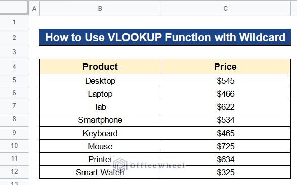
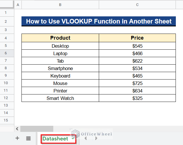
Let’s get introduced to our dataset first. Here we have some products in Column B and their prices in Column C. With the help of this dataset, I’ll show you 2 suitable examples to use the VLOOKUP function with Wildcard in Google Sheets. Let’s see how to do it.

Example 1: Using VLOOKUP Function with Asterisk Wildcard

We can use the VLOOKUP function with the Asterisk Wildcard (*) to fulfill different criteria. We can insert the Asterisk Wildcard (*) into the VLOOKUP formula to match something partially and get the output quickly. Let’s see 4 kinds of application of it.

1.1: Specific Characters at Starting

In the first case, we have some specific characters at starting position. The character is “Sma”. We want to look up this character in our dataset among the products and get the output as price. So we just simply put the Asterisk Wildcard (*) after this character and put it into our formula. Let’s see the steps below.

Steps:

• Firstly, type the following formula in Cell C15–

• Secondly, hit Enter to get the related price.

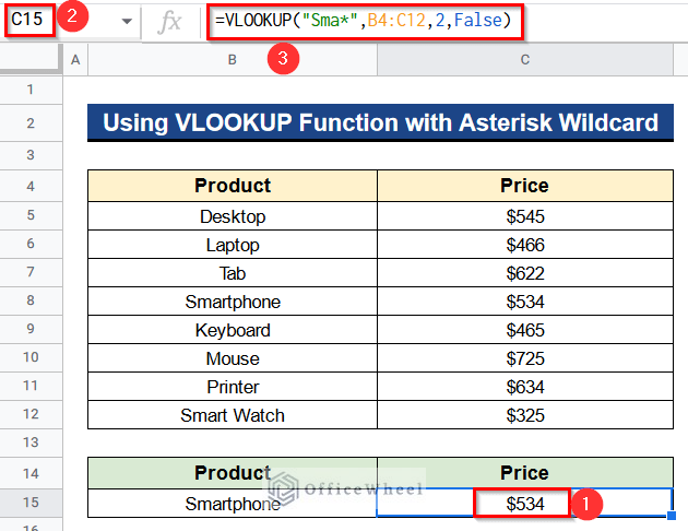
• Finally, you’ll see that the character “Sma” matches with Smartphone and gives its price.

1.2: Specific Characters at End

Now we’ll search for the value which has some specific characters at the end position. The character is “one”. We’ll just put the Asterisk Wildcard (*) before this character and put it into our formula.

Steps:

• At first, write the following formula in Cell C15–

• Then, press Enter to get the output.

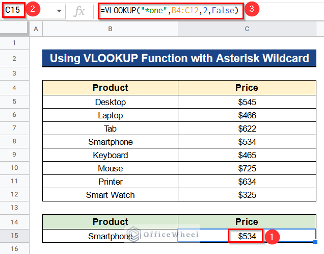
• Ultimately, you’ll notice that the character “one” match with Smartphone and gives its price.

1.3: Any Characters in Range

For this example, we have some characters which are the middle characters of any word. So we’ll use these characters to look up some values in our dataset. The characters are “tph”. Now we’ll put the Asterisk Wildcard (*) before and after these characters.

Steps:

• First, insert the following formula in Cell C15–

• Next, click Enter to get the result.

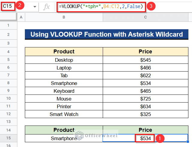
• At last, you may find that the characters match with Smartphone and gives its price.

1.4: Join Any Cell with Asterisk Wildcard

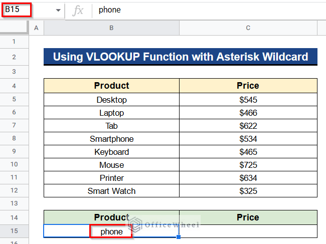
We have a different situation now. We have a dataset that has a value in Cell B15 as you can see in the picture. The value is partial. We have to match it with our product list. For this purpose, we can use the Asterisk Wildcard (*) and the & Sign together and add them before Cell B15 in our formula. Let’s see how to do it.

Steps:

• First of all, put the following formula in Cell C15–

• After that, hit the Enter Button to get the desired value.

• In the end, the value phone matches with Smartphone and gives its price.

Similar Readings

• Create Hyperlink to VLOOKUP Cell in Multiple Rows in Google Sheets
• How to Use VLOOKUP for Conditional Formatting in Google Sheets
• [Solved!] VLOOKUP Function Is Not Working in Google Sheets
• How to Use VLOOKUP with IF Statement in Google Sheets
• Use VLOOKUP with Drop Down List in Google Sheets

Example 2: Applying VLOOKUP Function with Question Mark Wildcard

Additionally, we may use the Question Mark Wildcard (?) with the VLOOKUP function to match any single character. Now we’ll search for the product Tab but will omit the character “b” from it. We’ll place a Question Mark Wildcard (?) in place of character “b”. You’ll be surprised to see that the result will be automatic.

Steps:

• In the first place, type the following formula in Cell C15–

• Afterward, press the Enter Button to get the desired output.

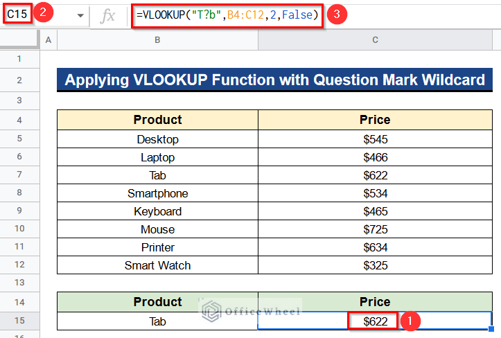
• Again, you can see that the formula is giving the price of Tab.

Read More: How to VLOOKUP Between Two Google Sheets (2 Ideal Examples)

How to Use REGEXMATCH Function Instead of Wildcard in VLOOKUP Range in Google Sheets

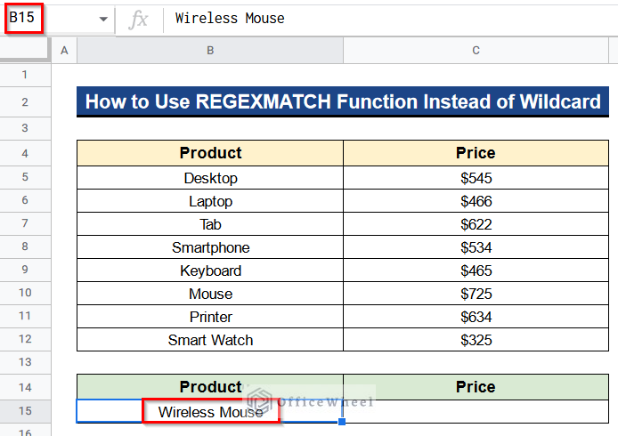
Apart from all the above-mentioned methods, we can use the combination of the REGEXMATCH, FILTER and INDEX functions to partially match something in our dataset. These functions serve the same purpose that the VLOOKUP function with Wildcard serves. We’ll search for the value in Cell B15 in our dataset. Below you’ll find the steps for doing so.

Steps:

• In the beginning, write the following formula in Cell C15–

• Consequently, click the Enter Button to get the desired price.

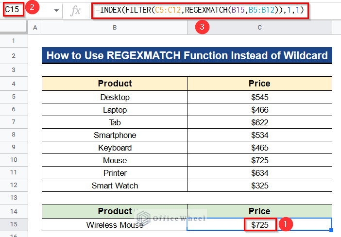
• Lastly, you may see that the value was Wireless Mouse. But it matches with Mouse and gives its price. So it is a partial match.

Read More: How to VLOOKUP All Matches in Google Sheets (2 Approaches)

How to Use VLOOKUP Function with Wildcard in Another Google Sheets

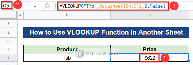
Sometimes we need to use the VLOOKUP function with Wildcard from one sheet to another Google Sheets. Here I’ll show that procedure with some simple steps. I am using the Question Mark Wildcard (?) for this reason. You can also do this with other Wildcards.

Steps:

• Before all, rename the sheets as Datasheet.

• Moreover, go to another sheet and insert the following formula in Cell C5–

• Ultimately, hit Enter to get the result in another sheet.

Read More: Alternative to Use VLOOKUP Function in Google Sheets

Conclusion

That’s all for now. Thank you for reading this article. In this article, I have discussed 2 useful examples to use the VLOOKUP function with Wildcard in Google Sheets. I have also discussed using the REGEXMATCH function instead of Wildcard in the VLOOKUP range in Google Sheets. Moreover, I have talked about using the VLOOKUP function with Wildcard in another Google Sheets. Please comment in the comment section if you have any queries about this article. You will also find different articles related to google sheets on our officewheel.com. Visit the site and explore more.

Related Articles

• Google Sheets Vlookup Dynamic Range
• How to Use VLOOKUP with Named Range in Google Sheets
• Use Nested VLOOKUP in Google Sheets
• How to Check If Value Exists in Range in Google Sheets (4 Ways)
• VLOOKUP Error in Google Sheets (with Quick Solutions)
• VLOOKUP with IMPORTRANGE Function in Google Sheets
• How to VLOOKUP Multiple Columns in Google Sheets (3 Ways)
• Use VLOOKUP to Import from Another Workbook in Google Sheets