Merging cells in a spreadsheet is one of the more fundamental skills to have. But things might get complex when certain patterns of merges are involved. So today, we will be looking at how to merge rows in Google Sheets.
We have created this comprehensive guide, giving examples of processes that users of every level of spreadsheet expertise can use.
3 Ways of How to Merge Rows in Google Sheets
1. Merge Rows from Toolbar
Let’s start with the most common way to merge cells in general in Google Sheets, that is from the Toolbar menu.
You can find the Merge cells button right above the Formula Bar:
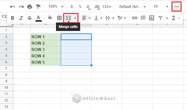
Now, for our selection in the worksheet, clicking on the Merge cells button will merge the rows. But if we had more than one column selected, both the columns and the rows would have been merged.
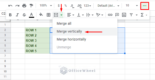
So, to specifically merge rows in Google Sheets, we need to Merge Vertically.
We can access this option by clicking on the drop-down icon beside the Merge cells button. Here you’ll find Merge vertically.
Our result:
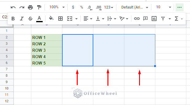
As you can see, all the rows have been merged, but the columns have remained unchanged.
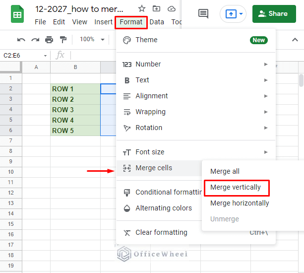
You can access the same option from the Format bar up top:
Format > Merge cells > Merge vertically
Data Loss
So far, we have worked on merging rows with empty cells. Things get a little hairy when we go to merge cells with values in them. These values can be raw data, formulas, or even whitespaces.
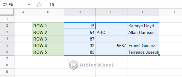
Let’s see what happens when we populate the cells and try to merge in the process we have just discussed.
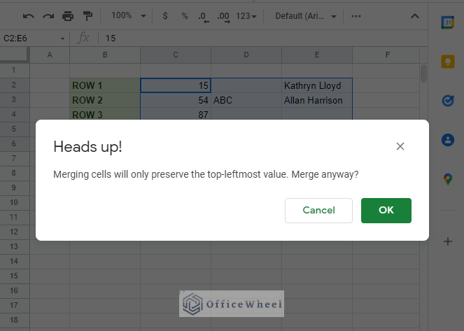
When we click on the Merge vertically button, we are hit with the following warning:
The result after we click OK:
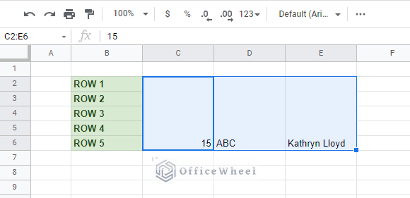
Only the topmost values remain, the rest of them have been wiped out.
Even after we Unmerge, the values don’t return.
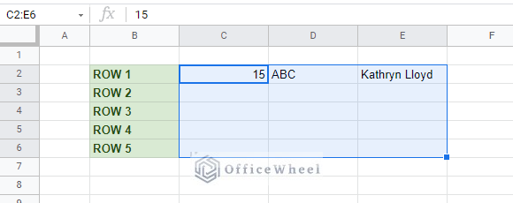
We have no choice but to Undo to get our values back.
This is one of the biggest weaknesses of the automatic Merge cells option in Google Sheets.
But worry not! We have workarounds where you can easily merge rows without losing data discussed in the next section, including a special add-on feature.
2. Merge Rows with Formula (Without Data Loss)
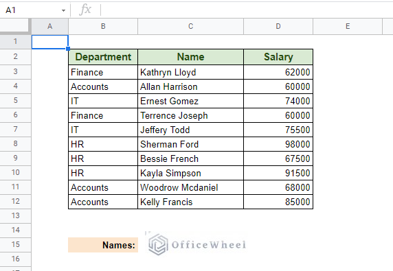
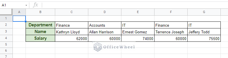
For this section, we will be using the following worksheet.
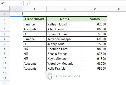
Here we have three columns – Department, Name, and, Salary of employees.
Our task is to merge or combine the rows of data according to their department.
I. Using the CONCATENATE Function
The first function we are going to use is the CONCATENATE function. It is self-explanatory.
For this example, we will be combining the Names and Salaries of the employees of the IT Department. We have two instances of it, one in row 5 and the other in row 7.
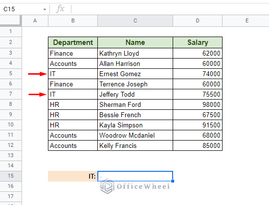
Let’s enter our formula in cell C15:
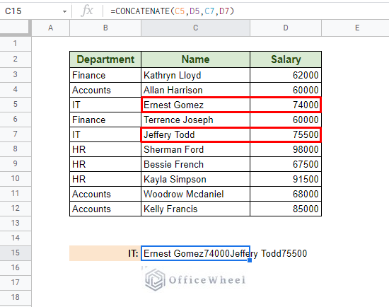
Now, this doesn’t look very appealing.
So let’s add some text modifications to our combination:
=CONCATENATE(C5," (",D5,"), ",C7," (",D7,")")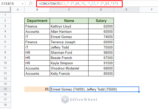
We have simply added parentheses for the salaries and spaces to go in between. Any text or string additions in the CONCATENATE function are treated as separate entities and must be enclosed in quotation marks (“”).
II. Using the JOIN Function
When you have a common delimiter or separator, the JOIN function performs better than the CONCATENATE function.
The JOIN function takes the delimiter separately making it the ideal function to make lists.
So as an example, we will be merging all the rows under the Name column and making a list of names below the table.
Our formula at C15 will be:
=JOIN(", ",C3:C12)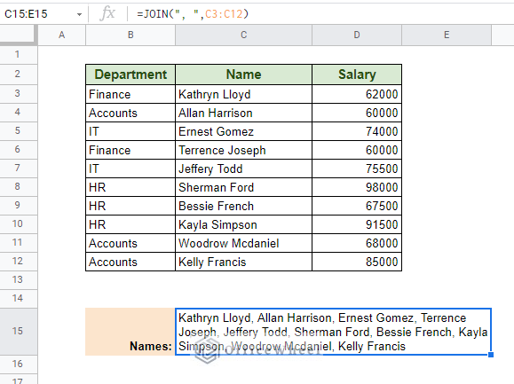
Cleaning Up Our Presentation
Practically speaking, combining rows will not be as simple as listing names in one cell. For that, let’s take the help of two other functions of Google Sheets to list the Names according to the Department. This should add another layer of complexity.
The first function we are going to be using is UNIQUE. We will use it to list the different departments from our table.
Our formula at B15:
=UNIQUE(B3:B12)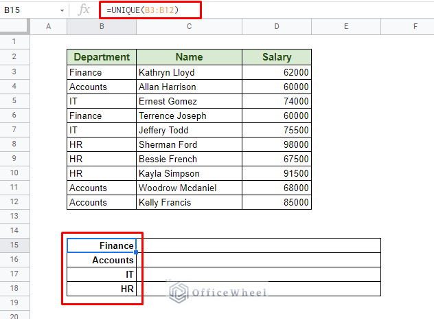
This column acts as a reference for our main JOIN formula, where we will be adding another function called FILTER.
The formula at C15:
=JOIN(", ",FILTER($C$3:$C$12,$B$3:$B$12=B15))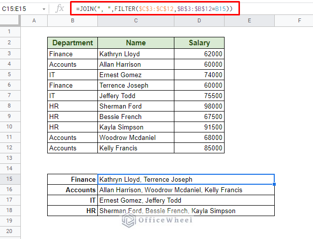
The FILTER function within the JOIN takes reference from the UNIQUE column to extract data from the Name column.
We have also locked our FILTER ranges with absolutes ($) as we don’t want it to move around as we use the fill handle or copy-paste formulas.
3. Merge Rows Using Add-Ons
Going back to our data loss argument in method 1, we mentioned that we can’t merge cells in place without losing data.
What if we say that we can overcome that issue in less than 5 minutes?
We will do this by using an add-on extension for Google Sheets called Merge Values.
How to Get
Navigate to the Extensions tab > Add-ons > Get add-ons
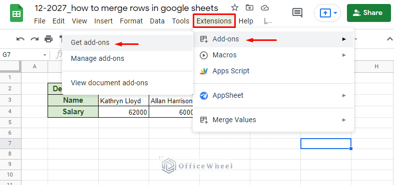
This should open the Extensions marketplace. Here, simply search for Merge Values and install. It’s free!

Using the Merge Values Add-on
We will be merging our rows in the following worksheet. It is simply a transposed version of our original table, transformed to better present the merging of rows with the add-on.
We will be guiding you through the procedure step-by-step:
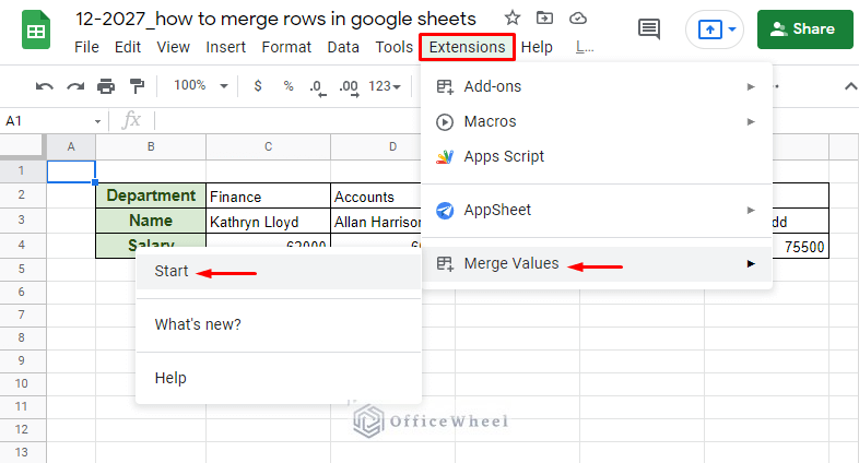
Step 1: Highlight your table and open the Merge Values add-on: navigate to Extensions > Merge Values > Start
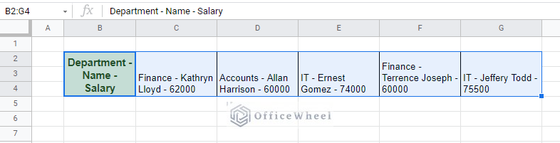
Step 2: Select these options in the Merge Values menu tray:
- in each selected column: This is the merge rows option for the add-on.
- [Space]-[Space]: This is our delimiter. In text form:
“ – " - top cell: This is where the results will be placed.
- Merge cells in each column: The merge will occur within the selected range. Another row will not be created.
- Wrap text: Optional. The merge will not breach the cell’s boundaries.
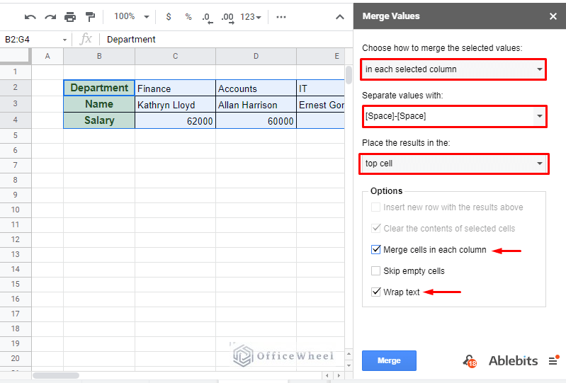
Step 3: Click Merge.
A word of advice: Create a backup of your data before using this add-on, especially if you are a free user since the add-on does not allow you to roll back changes. Subscribed users will have the option to backup the entire worksheet in the Options menu.
Final Words
We hope that all the methods for merging rows in Google Sheets come in handy for your spreadsheet tasks. We understand that the task of merging cells is fundamental and have tried to present a way for every level of spreadsheet expertise.
However, for a simple merge, please follow the How to Merge Cells in Google Sheets article.
Feel free to post any queries or advice you might have in the comments section.