We often need to insert values into a cell based on other cells in Google Sheets. Also, finding information in a large spreadsheet takes a lot of work. However, you can find information based on values in another cell. In this article, I’ll discuss 7 helpful methods to form formulas in Google Sheets if a cell contains specific text and then return value in another cell.
A Sample of Practice Spreadsheet
You can copy our practice spreadsheets by clicking on the following link. The spreadsheets contain an overview of the datasheet and an outline of the described methods to form formulas in Google Sheets if the cell contains specific text and then return the value in another cell.
7 Methods to Return Value in Another Cell If Cell Contains Text in Google Sheets
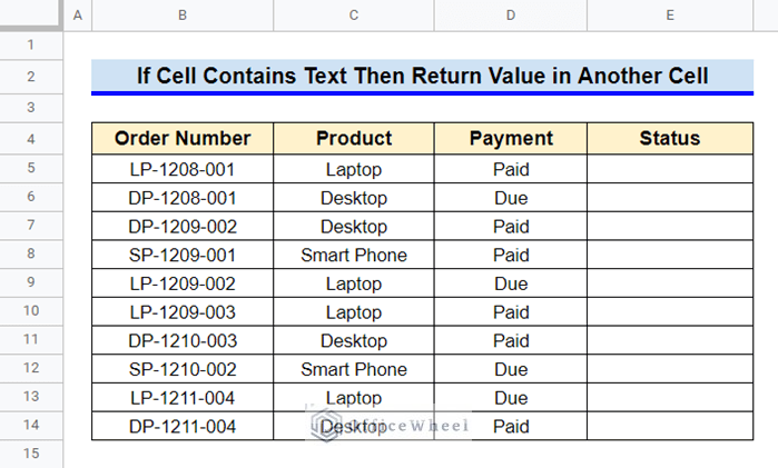
First, let’s get familiar with our datasheet. It contains the order number, product name, and payment status for several customer orders. We’ll set the order status as “Confirm” or “Pending” based on subsequent payment status.
1. Using IF Function
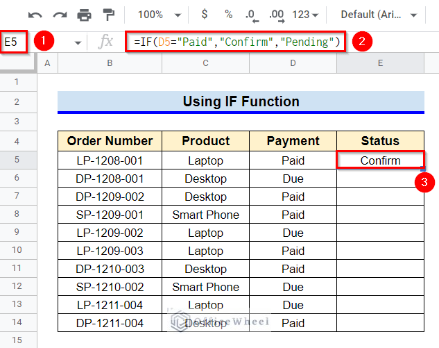
We can simply use the IF function to test whether the payment status is “Paid” or “Due” and return values in another cell accordingly.
Steps:
- First, select Cell E5 and then type in the following formula-
=IF(D5="Paid","Confirm","Pending")- After that, press Enter key to get the required value.
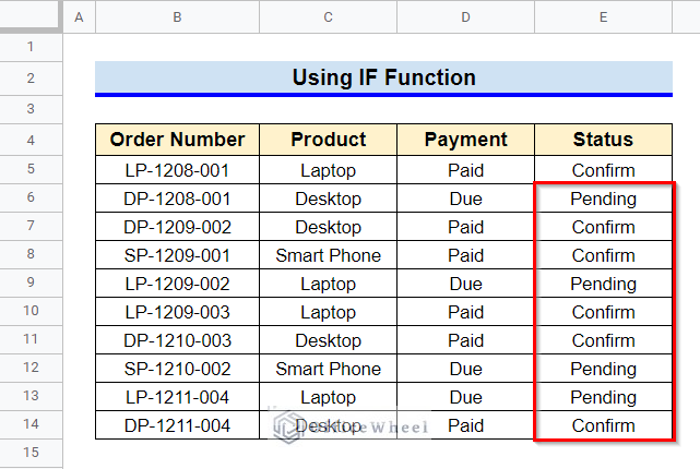
- Point your mouse to the lower right corner of Cell E5 to view the Fill Handle Drag the Fill Handle icon up to Cell E14 to get values for other cells of Column E.

- Thus we can return values in cells of Column E based on text values in cells of Column D.
Read More: How to Use ARRAYFORMULA with IF Function in Google Sheets
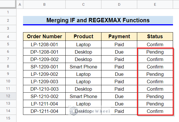
2. Merging IF and REGEXMAX Functions
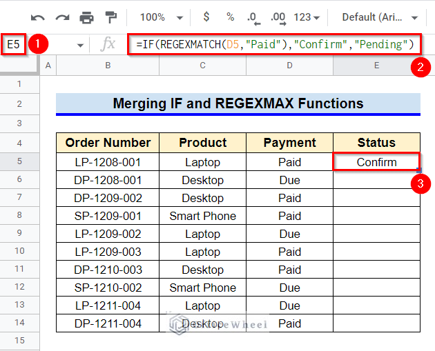
We can merge the REGEXMAX function with the IF function to perform the logical test and then return values in a cell if another cell contains a specific test.
Steps:
- Select Cell E5 first and then type in the following formula-
=IF(REGEXMATCH(D5,"Paid"),"Confirm","Pending")- After that, press Enter key to get the required text value.
Formula Breakdown
- REGEXMATCH(D5,”Paid”)
First, the REGEXMATCH function checks whether Cell D5 contains the string “Paid” and then returns TRUE if a match is found. Else, it returns FALSE.
- IF(REGEXMATCH(D5,”Paid”),”Confirm”,”Pending”)
Finally, the IF function returns “Confirm” if a match is found in the logical test. Else, it returns “Pending”.
- Finally, use the Fill Handle icon to fill values in other cells of Column E.
Read More: Highlight Cell If Value Exists in Another Column in Google Sheets
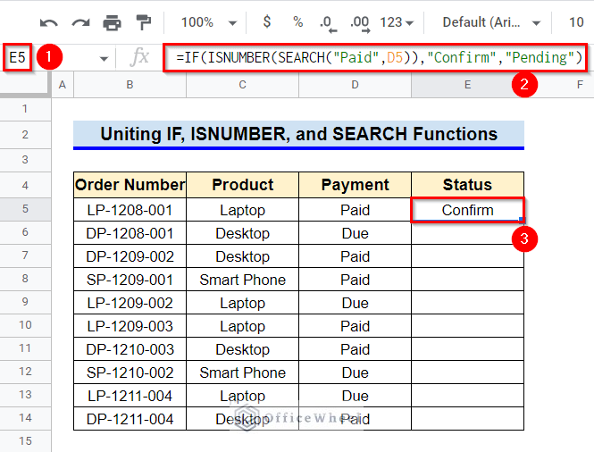
3. Uniting IF, ISNUMBER, and SEARCH Functions
Another way to perform the logical test in the IF function is to unite it with the ISNUMBER and SEARCH functions.
Steps:
- First, select Cell E5 and type in the following formula-
=IF(ISNUMBER(SEARCH("Paid",D5)),"Confirm","Pending")- Afterward, press the Enter key to get the required text.
Formula Breakdown
- SEARCH(“Paid”,D5)
First, the SEARCH function searches for the string “Paid” in Cell D5. If the string is found, it returns the position (a number) where the string is in Cell D5. Else, it returns #Value! error which is a text.
- ISNUMBER(SEARCH(“Paid”,D5))
Afterward, if the SEARCH function finds a match and returns a number, the ISNUMBER function returns TRUE. Else, it returns FALSE.
- IF(ISNUMBER(SEARCH(“Paid”,D5)),”Confirm”,”Pending”)
Finally, the IF function returns “Confirm” if the logical expression is true. Else, it returns “Pending”.
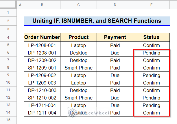
- Finally, use the Fill Handle icon to get values in other cells of Column E.
Read More: How to Use Multiple IF Statements in Google Sheets (5 Examples)
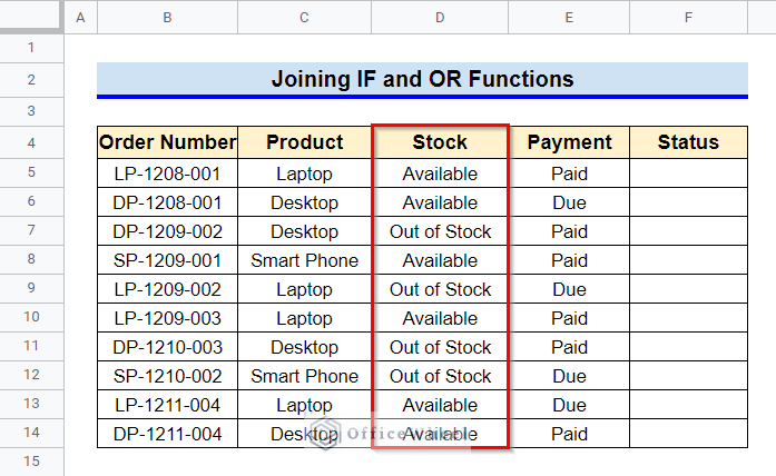
4. Joining IF and OR Functions
If you want to return values based on text values in multiple cells, you can use the OR function and the AND function. The OR and AND functions can be applied alongside any of the previous three methods.
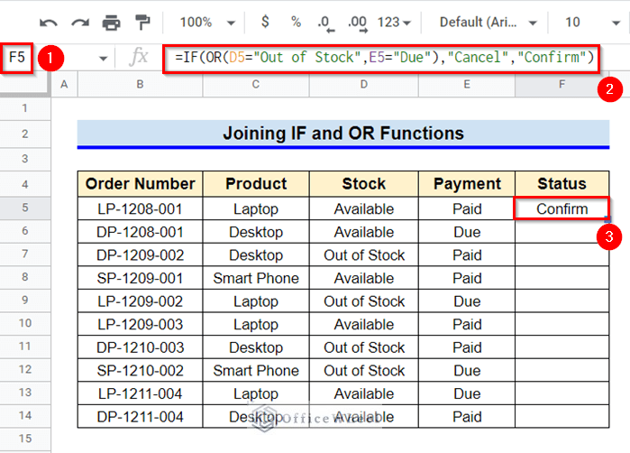
Here, I’ll be joining the IF and OR functions. I have made some changes to the datasheet too. A new column titled Stock is added. I’ll cancel the order if a product is out of stock or the payment is due. Otherwise, I’ll confirm the order.
Steps:
- First, select Cell F5.
- After that, type in the following formula-
=IF(OR(D5="Out of Stock",E5="Due"),"Cancel","Confirm")- Press the Enter key to get your required result.
Formula Breakdown
- OR(D5=”Out of Stock”,E5=”Due”)
First, the OR function checks the criteria at Cell D5 and E5. If none of the criteria matches, then the OR function returns FALSE. Otherwise, it returns TRUE.
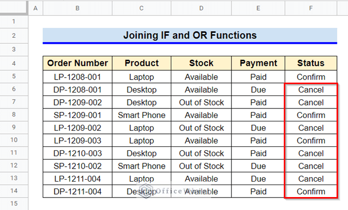
- IF(OR(D5=”Out of Stock”,E5=”Due”),”Cancel”,”Confirm”)
After that, the IF function returns “Cancel” if the logical expression is true. Else, it returns “Confirm”.
- Finally, use the Fill Handle icon to get values in other cells of Column F.
Read More: How to Use IF and OR Formula in Google Sheets (2 Examples)
5. Combining IF and AND Functions
Combining the AND function with the IF function is very similar to the joining of the OR and IF functions. Although, unlike the OR function, the AND function returns TRUE when both criteria match. So, there will be a slight change from the previous method in the formation of the formula.
Steps:
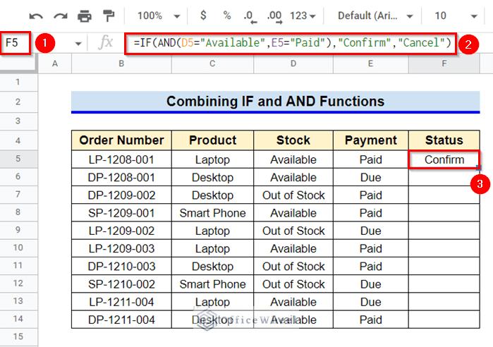
- First, select Cell F5.
- After that, type in the following formula-
=IF(AND(D5="Available",E5="Paid"),"Confirm","Cancel")- Press the Enter key to get your required result.
Formula Breakdown
- AND(D5=”Available”,E5=”Paid”)
To start with, the AND function checks the criteria at Cell D5 and E5. If both the criteria match, the AND function return TRUE. Else, it returns FALSE.
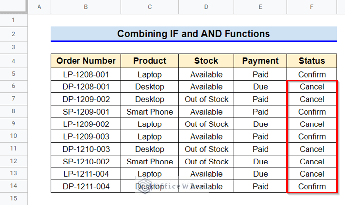
- IF(AND(D5=”Available”,E5=”Paid”),”Confirm”,”Cancel”)
Finally, the IF function return “Confirm” if the logical test is true, else it returns “Cancel”.
- Finally, use the Fill Handle icon to fill other cells in Column F.
Read More: Conditional Formatting with Multiple Conditions Using Custom Formulas in Google Sheets
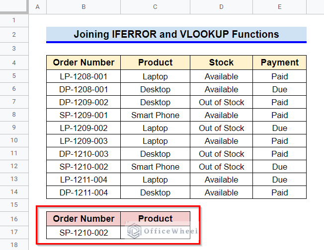
6. Joining IFERROR and VLOOKUP Functions
If you simply want to search values in a datasheet based on specific values from a cell, you can use the VLOOKUP function. For example, we want to extract the product name for any order number. Change the dataset to the following for that. As we can see, one cell contains the order number in Cell B17. Now, we will return the product name in Cell C17 using the VLOOKUP function.
Steps:
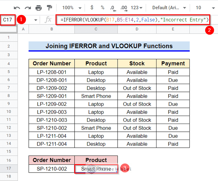
- First, select Cell C17.
- After that, type in the following formula:
=IFERROR(VLOOKUP(B17,B5:E14,2,False),"Incorrect Entry")- Finally, press Enter key to get the required text value.
Formula Breakdown
- VLOOKUP(B17,B5:E14,2,False)
The VLOOKUP function searches down the first column of the range B5:E14 for the search key specified by Cell B17 and returns the value from column 2 of the range in the row where a match is found.
- IFERROR(VLOOKUP(B17,B5:E14,2,False),”Incorrect Entry”)
If the VLOOKUP function doesn’t find a match, then the IFERROR function returns the string “Incorrect Entry”.
Read More: How to Use VLOOKUP for Conditional Formatting in Google Sheets
Similar Readings
- Google Sheets: Conditional Formatting Row Based on Cell
- How to Highlight Row If Cell Is Not Empty in Google Sheets
- Highlight Row Based on Date in Google Sheets (2 Suitable Ways)
- Filter Values that Contains Multiple Text Criteria in Google Sheets (2 Easy Ways)
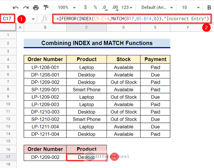
7. Combining INDEX and MATCH Functions
An alternative to the VLOOKUP function is to combine the INDEX and MATCH functions. We’ll also use the IFERROR function in case incorrect entries are made.
Steps:
- Select Cell C17.
- Then, type in the following formula:
=IFERROR(INDEX(C5:C14,MATCH(B17,B5:B14,0)),"Incorrect Entry")- Press Enter key finally to get the required result.
Formula Breakdown
- MATCH(B17,B5:B14,0)
First, the MATCH function returns the relative position of the search key specified by Cell B17 in the range B5:B14.
- INDEX(C5:C14,MATCH(B17,B5:B14,0))
Then, the INDEX function returns the content of the cell in the relative position returned by the MATCH function from range C5:C14.
- IFERROR(INDEX(C5:C14,MATCH(B17,B5:B14,0)),”Incorrect Entry”)
Finally, if any error occurs in the INDEX and MATCH functions, the IFERROR function returns the string “Incorrect Entry”.
Read More: Match Multiple Values in Google Sheets (An Easy Guide)
Things to Be Considered
- The VLOOKUP function is not case-sensitive.
- If the dataset is not sorted while using the VLOOKUP function, then let Google Sheets know about it by specifying the fourth argument as False or 0.
Conclusion
This concludes our article on how to form a formula in Google Sheets if a cell contains text and then return a value in another cell. I hope the described methods were sufficient for your requirements. Feel free to leave your thoughts on the article in the comment box. Visit our website OfficeWheel.com for more helpful articles.
Related Articles
- How to Do IF THEN in Google Sheets (3 Ideal Examples)
- Google Sheets: Conditional Formatting with Multiple Conditions
- How to Use Nested IF Statements in Google Sheets (3 Examples)
- Google Sheets IF Statement in Conditional Formatting
- Use Nested IF Function in Google Sheets (4 Helpful Ways)
- How to Use IF Condition Between Two Numbers in Google Sheets