Users who frequently work with huge spreadsheets may wish to look for a value that belongs to a specific category and doing so manually might be time-consuming. To accomplish this, we can utilize the HLOOKUP function. HLOOKUP is an abbreviation for Horizontal Lookup. The function looks for a specified value in the first row of the input range and returns the value of a specific cell in the column where the specified value is located. We can look for a value based on multiple criteria in Google Sheets using the HLOOKUP function. In this article, I will show 2 simple ways of using the HLOOKUP function for multiple criteria in Google Sheets.
2 Simple Ways to Use HLOOKUP Function for Multiple Criteria in Google Sheets
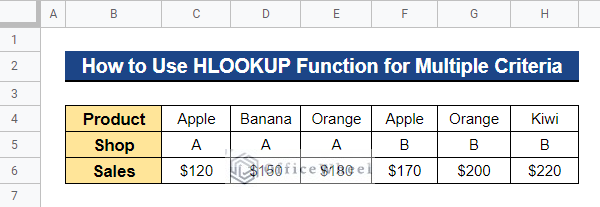
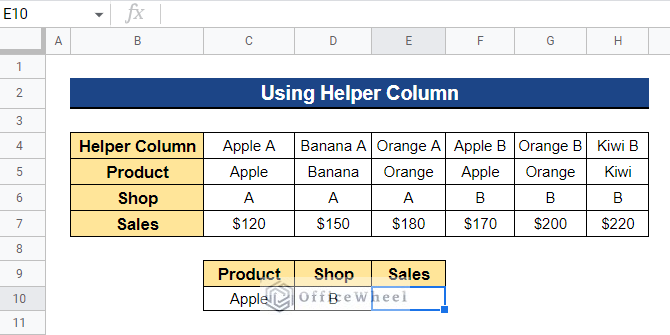
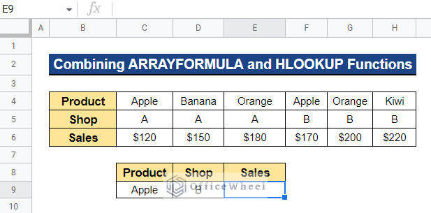
We will use the dataset below to demonstrate 2 simple ways of using the HLOOKUP function for multiple criteria in Google Sheets. The dataset contains Product names from two distinct shops, as well as product Sales from those shops. Now we’ll search for a specific product sales value from a particular shop.
1. Using Helper Column
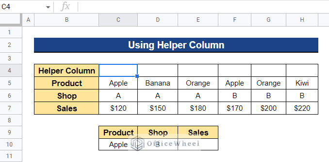
The first way includes the inclusion of a Helper column, which will contain a mixture of the criterion fields. In our case, we may place the Helper row on top of the Product row, making it the first row of the search range. The Helper row has a space-separated combination of the Product and Shop names for each column. With the help of the Helper column, we will look for a specific value in our data range using the HLOOKUP function in Google Sheets.
Steps:
- Firstly, select the first cell of the Helper row, we selected Cell C4.
- Next, input the formula below and press Enter–
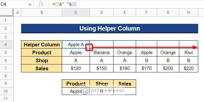
=C5&" "&C6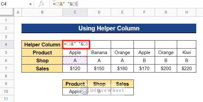
- Thus, it will combine Cell C5 and Cell C6. Now, to apply the formula to the remaining cells, drag the Fill Handle icon rightward.
- After that, with the help of the Helper column, we will search for a value based on multiple criteria. Choose the cell first to which you’re going to apply the formula to look for a specific value. We chose Cell E10.
- Next, enter the following formula and hit Enter–
=HLOOKUP(C10&" "&D10,C4:H7,4,FALSE)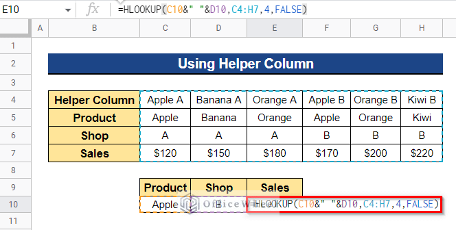
- Thus, it will display the product sale based on Cell C10 and Cell D10.
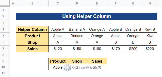
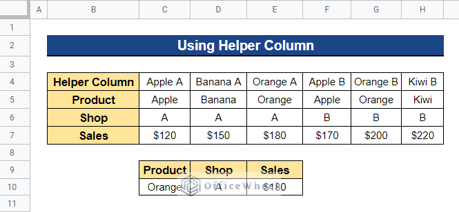
- Here, we changed the lookup values and see, it’s showing the corresponding accurate result.
2. Combining ARRAYFORMULA and HLOOKUP Functions
This strategy accomplishes the same task as the first. The only change is that the helper column is produced dynamically this time, rather than needing to physically build an additional column for it. The approach used the ARRAYFORMULA function to construct a virtual table to search for.
Steps:
- Firstly, choose a cell to which you will apply the formula to search for a specific value based on multiple criteria. In our case, we chose Cell E9.
- Now, enter the following formula and press the Enter button-
=ARRAYFORMULA(HLOOKUP(C9&" "&D9, {C4:H4&" "&C5:H5;C6:H6},2,FALSE))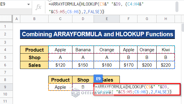
Formula Breakdown
- ARRAYFORMULA(HLOOKUP(C9&” “&D9, {C4:H4&” “&C5:H5;C6:H6},2,FALSE))
First, the ARRAYFORMULA function will make an array of cells combining Row 4 and Row 5 of the data range.
- HLOOKUP(C9&” “&D9, {C4:H4&” “&C5:H5;C6:H6},2,FALSE)
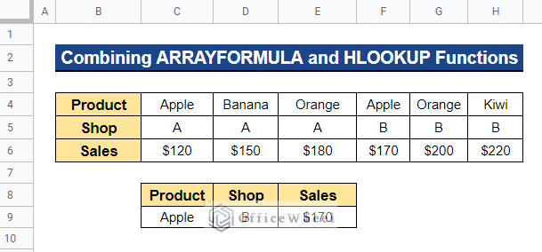
Then, the HLOOKUP function searches the combination of Cell C9 and Cell D9 among the array and returns the value of the last row.
- As a result, it will show the product sale based on Cell C10 and Cell D10.
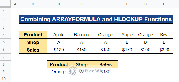
- We inserted another set of lookup values here, and it’s giving the proper output like the previous method.
How to Combine VLOOKUP and HLOOKUP Functions to Do 2D Searches in Google Sheets
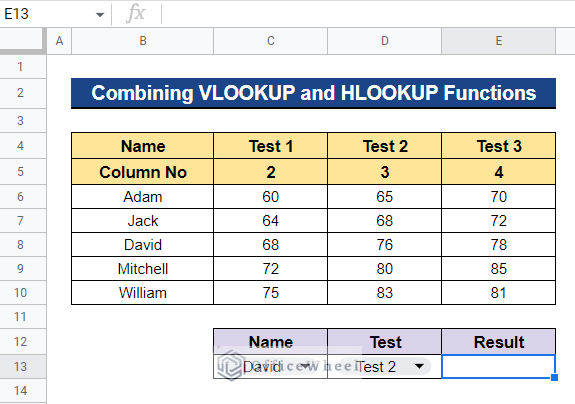
VLOOKUP and HLOOKUP are two of the most often used functions in Google Sheets. VLOOKUP conducts vertical searches, whereas HLOOKUP does horizontal searches. In Google Sheets, combining VLOOKUP and HLOOKUP may be quite effective. They may be combined to do 2D table searches. Assume we have a list of students and their scores from three tests. We wish to look for a particular test result from a specific student.
Steps:
- First, select a cell to which you want to apply the formula, we selected Cell E13. Our lookup values are in Cell C13 and Cell D13, and we’ve utilized a drop-down validation rule in the lookup cells to make our worksheet dynamic.
- Now, type the formula below and hit the Enter key-
=VLOOKUP(C13,B6:E10,HLOOKUP(D13,C4:E5,2,FALSE),FALSE)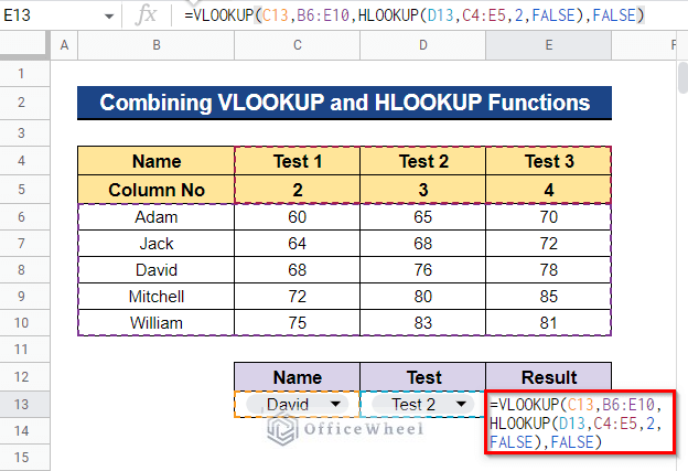
Formula Breakdown
- HLOOKUP(D13,C4:E5,2,FALSE)
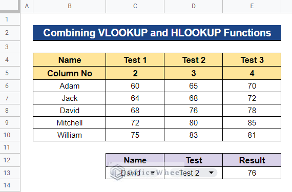
First, the HLOOKUP function will search Cell D13 among the first row of the data range Cell C4:E5 and it will return the value of the second row of the data range that will work as the column index for the VLOOKUP function.
- VLOOKUP(C13,B6:E10,HLOOKUP(D13,C4:E5,2,FALSE),FALSE)
Then, the VLOOKUP function will look for Cell C13 among the data range Cell B6:E10 and it will return the value of that column of the data range that is specified by the HLOOKUP function.
- Thus, it will display the result of a specific test taken by a specific student.
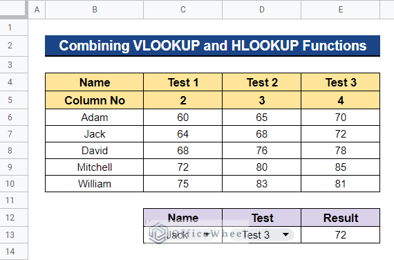
- We updated the lookup values and now it displays the corresponding accurate result.
Read More: Combine VLOOKUP and HLOOKUP Functions in Google Sheets
Conclusion
In this article, I demonstrated two simple ways to use the HLOOKUP function in Google Sheets for multiple criteria. I also demonstrated how to use the VLOOKUP and HLOOKUP functions in tandem to do 2D table searches. Please leave any questions or suggestions in the comments section below. Visit Officewheel.com to discover more.