There are several functions like STDEV, STDEVA, STDEVP, etc. in Google Sheets that can measure the standard deviation for a range. These functions take a numerical data range as input and return the standard deviation of that data range. Sometimes, the data range we provide may contain 0 values. There can be several reasons behind a 0 value, but often we enter a 0 value for inappropriate cases. Therefore, including the cell in a data range may cause the mentioned functions to return a standard deviation that doesn’t express the actual spread of given data. Hence, the question arrives: “Can we use the Standard Deviation formula ignoring 0 values?”. The answer is a resounding Yes! And in this article, I’ll demonstrate 3 simple ways to ignore 0 values while using a Standard Deviation formula (the STDEV formula) in Google Sheets.
A Sample of Practice Spreadsheet
You can copy our practice spreadsheets by clicking on the following link. The spreadsheet contains an overview of the datasheet and an outline of the described ways to use the Standard Deviation formula ignoring 0 in Google Sheets.
What Is Standard Deviation?
The standard deviation is a parameter in statistics to measure the amount of variation or dispersion in a given dataset. A lower standard deviation value indicates that the values of the dataset are closer to the mean value, while a higher standard deviation indicates that the values are in a wider span in that data range.
3 Simple Ways to Ignore 0 for Standard Deviation Formula in Google Sheets
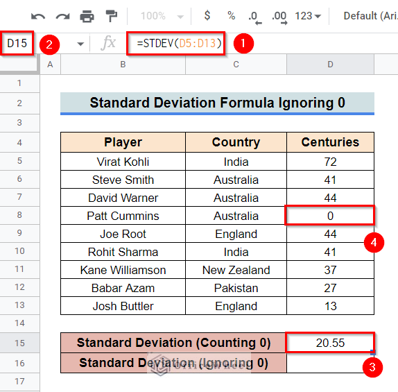
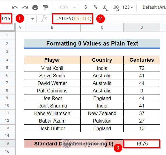
First, let’s get familiar with our dataset. The dataset contains a list of hundreds scored by several cricket players from various countries. The STDEV function is used for calculating the standard deviation of the given data in Cell D15. As you can see one of the players hasn’t scored any hundreds. Therefore, the standard deviation is quite high here. But since that player is not a proper batsman, including him in this range doesn’t provide an accurate insight into this data. Therefore, we’ll ignore the cells with a 0 value and calculate the standard deviation for the remaining cells. Keep reading to learn how.
1. Combining STDEV and FILTER Functions
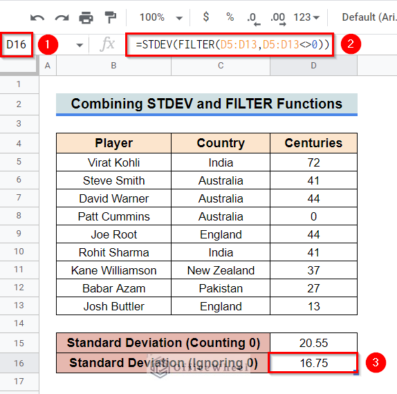
The FILTER function can be combined with the STDEV function to ignore cells with 0 values and return the standard deviation of the remaining cells.
Steps:
- First, select Cell D16.
- Afterward, type in the following formula-
=STDEV(FILTER(D5:D13,D5:D13<>0))- Finally, press Enter key to get the required result.
Formula Breakdown
- FILTER(D5:D13,D5:D13<>0)
First, the FILTER function returns the filtered version of the source data range D5:D13 by ignoring cells with 0 values.
- STDEV(FILTER(D5:D13,D5:D13<>0))
And then the STDEV function returns the standard deviation of the filtered range.
Read More: How to Add Different Standard Deviation Bars in Google Sheets
Similar Articles
- How to VLOOKUP Last Match in Google Sheets (5 Simple Ways)
- How to Calculate Weighted Average Using IF Function in Google Sheets
- How to VLOOKUP Multiple Columns in Google Sheets (3 Ways)
- How to Use the DATEVALUE Function in Google Sheets (An Easy Guide)
- How to Sum Using ARRAYFORMULA in Google Sheets
2. Uniting STDEV, ARRAYFORMULA, and IF Functions
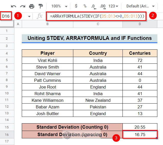
Another way to ignore 0 values while using the standard deviation formula STDEV is to combine it with the ARRAYFORMULA and IF functions.
Steps:
- First, select Cell D16.
- After that, type in the following formula-
=ARRAYFORMULA(STDEV(IF(D5:D13<>0,D5:D13)))- Finally, press Enter key to get the required standard deviation.
Formula Breakdown
- IF(D5:D13<>0,D5:D13)
First, the IF function returns any cell within the range D5:D13 if it is not equal to zero.
- STDEV(IF(D5:D13<>0,D5:D13))
After that, the STDEV function calculates the standard deviation of the cells returned by the IF function.
- ARRAYFORMULA(STDEV(IF(D5:D13<>0,D5:D13)))
Here, the ARRAYFORMULA function helps the non-array function IF to Deal with an array.
Read More: Calculate Standard Deviation with IF Condition in Google Sheets
3. Formatting 0 Values as Plain Text
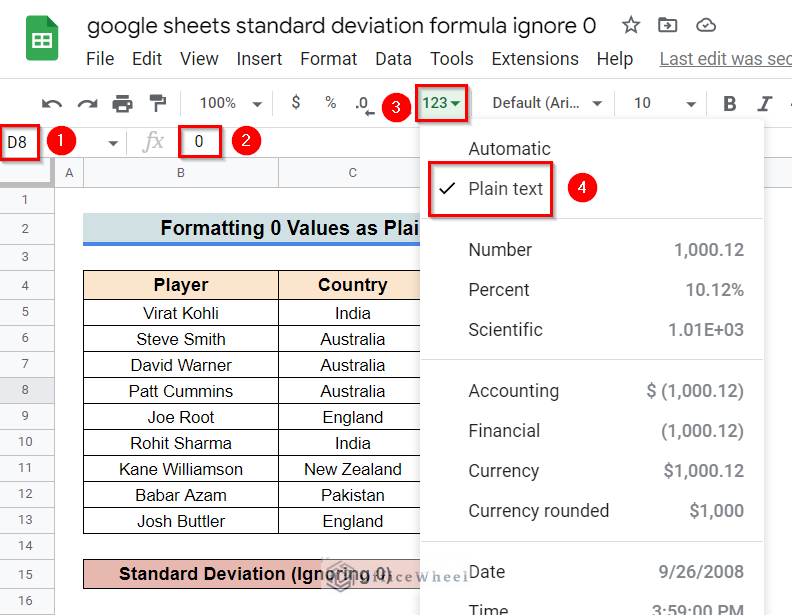
Perhaps, this is the simplest way to ignore 0 values while using the STDEV function. Since the STDEV function simply ignores text values, we can set plain text format for the cells that contain 0 values. However, for large datasets, many of the cells can contain 0 values. Therefore, manually changing the data format isn’t very efficient.
Steps:
- First, select all the cells with 0 values and set the data format as “Plain Text” from the menu options.
- Now, select Cell D15 and type in the following formula-
=STDEV(D5:D13)- Finally, press Enter key to get the required result.
Read More: Find the Top 10 Values in a Google Sheets Pivot Table (2 Easy Examples)
Things to Be Considered
- The IF function is a non-array function. Therefore, if want to enter an array as an argument for the IF function, unite the ARRAYFORMULA function with it.
- The STDEV function simply ignores text values.
Conclusion
This concludes our article to learn how to ignore 0 values while using a Standard Deviation formula in Google Sheets. I hope the demonstrated ways were sufficient for your requirements. Feel free to leave your thoughts on the article in the comment box. Visit our website OfficeWheel.com for more helpful articles.
Related Articles
- How to Link Cells Between Tabs in Google Sheets (2 Examples)
- How to Use IF and OR Formula in Google Sheets (2 Examples)
- Google Sheets Use Filter to Remove Duplicates in Column
- How to Use TRIM Function in Google Sheets (4 Easy Examples)
- How to Use Formula to Highlight Duplicates in Google Sheets
- How to Highlight Duplicates for Multiple Columns in Google Sheets
- How to Format Date with Formula in Google Sheets (3 Easy Ways)
- Calculate Standard Deviation of Weighted Variables in Google Sheets

