How to Highlight Duplicates for Multiple Columns in Google Sheets

Finding duplicate values is a simple and time-saving task in the present era of technology thanks to Google Sheets. Not only can we identify duplicates, but we can also highlight the data to make it more noticeable and usable. This post will demonstrate how to swiftly, accurately, and effortlessly highlight duplicates in multiple columns of Google Sheets.

A Sample of Practice Spreadsheet

3 Scenarios Where We Highlight Duplicates in Google Sheets for Multiple Columns

The data structure largely determines the scenarios. There can be 4 different approaches depending on how many columns or rows or what we’re looking for. A dataset of suitable examples is provided for each scenario about how to duplicate highlights in google sheet is detailed below.

1. Use COUNTIF Function and Conditional Formatting

First, there are a few techniques that focus on the impact on the rows of multiple columns.

1.1 In Multiple Columns

Imagine a database that contains a person’s incoming and outgoing calls. This process will identify names that appeared more than once in the table. These are the steps to find the duplicates.

Steps:

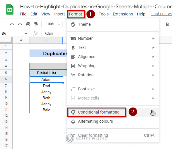
• Format > Conditional Formatting

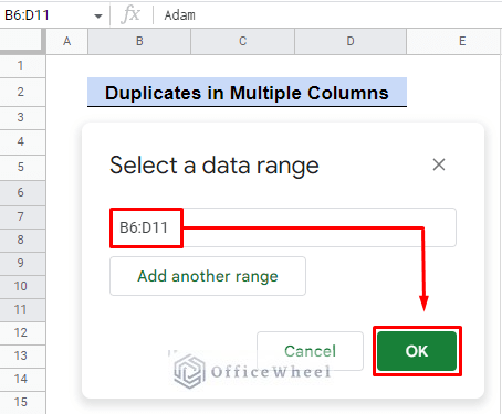
• Conditional Format Rules column > Apply to Range

• Set the data range as B6:D11. Don’t forget to press F4 in order to lock the range

• Select Format Rules > Custom formula is

• Now, we’ll enter the following formula in the empty space.

The COUNTIF functions in this case count the occurrences of the value B6 in the cells between B6 and D11. The formula can be improved by using “>1” so that it will only display the value if the count is more than 1.

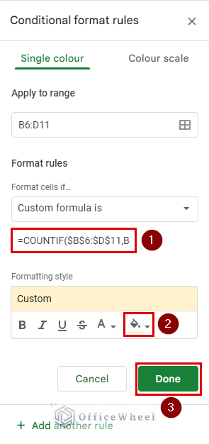
• For the cells to stand out, change the Fill color. We used light yellow in this case.
• Finally, click “Done”.

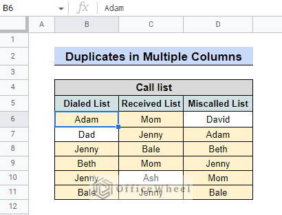
This scenario highlighted every cell with a duplicate value. David, Ash, and Dad only made one appearance in the dataset, which is why they weren’t given more attention.

Assume you’re curious about who you speak with the most. You establish a condition in order to discover that. For instance, the name should appear in the table more than four times. The updated formula will therefore be:

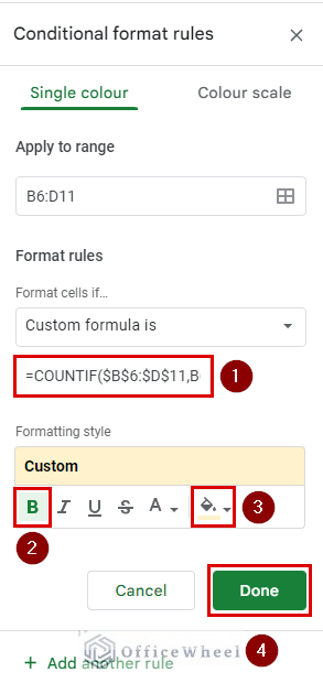
This time you will BOLD the cells for better visibility. Remember to change the Fill color, afterward click “Done“.

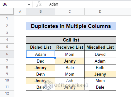
The table reveals that Jenny is the person you speak to the most frequently. She had five entries in the table with her name on them. It is one of the simple methods to Highlight Duplicates in Google Sheet in multiple columns.

Read More: Google Sheets: Conditional Formatting with Multiple Conditions

1.2 In Multiple Rows of Multiple Columns

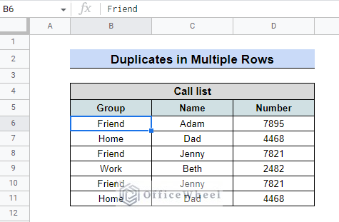
Suppose, there is a list of calls you get from your FRIEND, FAMILY, and WORK. Duplicates were made because you were trying to track down the callers who called you repeatedly. However, compared to the previous encounter, now you want to highlight the whole row rather than the individual cells for more information.

Steps:

• Up until the formula choice, the initial steps are the same as before.
• In the black space, we are going to use the following formula:

• BOLD the cells.
• Change the Fill color, for this example, the color is light yellow.
• Click “Done” to see the results.

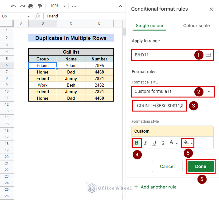
You can see that Dad and Jenny called you more than once at this table. Thus, it was possible to see the duplicate values in Google Sheets.

Read More: How to Sum Multiple Rows in Google Sheets (3 Ways)

Similar Readings

• How to Use IF and OR Formula in Google Sheets (2 Examples)
• Multi Row Dynamic Dependent Drop Down List in Google Sheets
• Google Sheets: Convert Text to Number (6 Easy Ways)
• Highlight Duplicates in Two Columns in Google Sheets (2 Ways)
• Conditional Formatting Based on Another Cell in Google Sheets

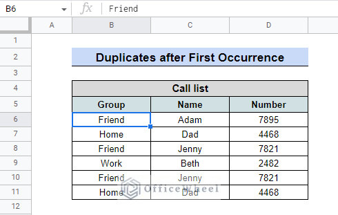
2. Highlight Duplicates after First Occurrence

In this scenario, You only desire to keep the first calls enlisted and learn about the later occurrences.

Same steps as before.

• Format > Conditional Formatting
• Conditional Format Rules column > Apply to Range
• Set the data range as B6:D11. Press F4 in order to lock the range
• Select Format Rules > Custom formula is

However, there is a slight change in the formula. This time we will use COUNTIF with ARRAYFORMULA to search in all the individual columns. ARRAYFORMULA force COUNTIF to look into each column to find a specific match.

Formula:

• Alternate the Fill color. In this instance, we chose light yellow.
• Then click “Done.”

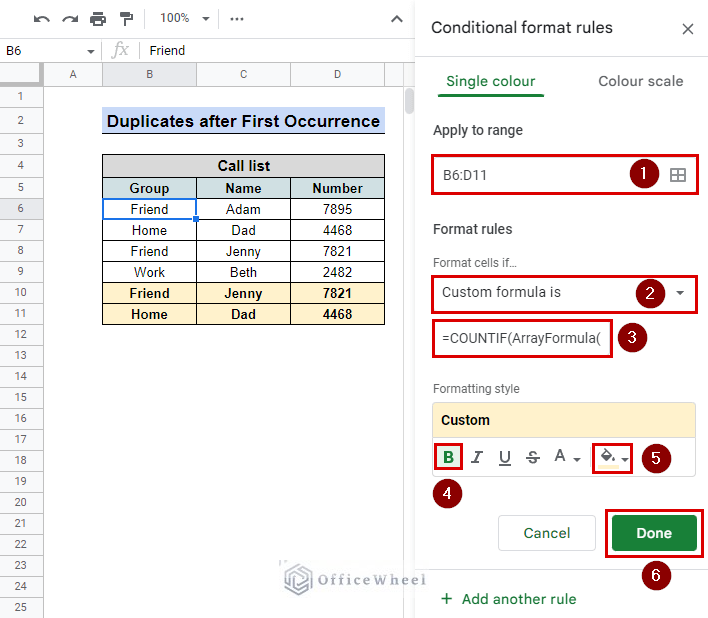
The formula notified you about all the entries as per your request, as you can see in the image, and did not highlight the first entry. Thus, you can highlight duplicates in Google Sheets in multiple columns after preserving the first occurrence.

Read More: How to Use ARRAYFORMULA in Google Sheets (6 Examples)

3. Duplicate Highlighting with Added Criteria

Take the example of your friend Jenny, who called you on both of her two numbers. Instead of only names, you should now focus on Number. With this in mind, you can add another requirement so that the formula can emphasize calls from the same individual using the same number.

Steps:

• Format > Conditional Formatting
• Conditional Format Rules column > Apply to Range
• Set the data range as B6:D11. To lock the range, press F4
• Select Format Rules > Custom formula is
• In order for COUNTIF to employ both criteria, the syntax needs to include the “*” (and) operator.

Formula:

• Change the Fill color. We used light yellow in this case.
• Finally, click “Done”.

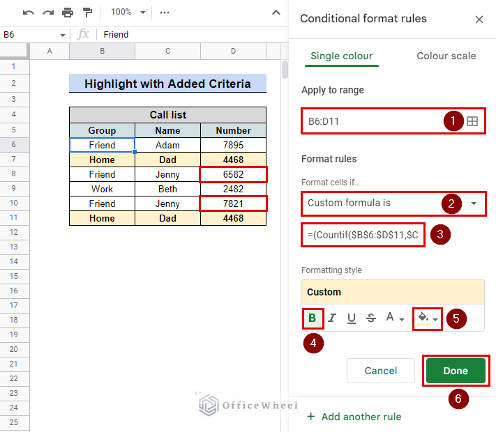
You see, Dad was the only one who met the requirements; thus, he was highlighted. Even though Jenny called twice as a duplicate value, her mismatched Number was excluded. You can include more criteria in order to filter more duplicates and highlight them in google Sheets multiple columns.

Read More: How to Use Formula to Highlight Duplicates in Google Sheets

Conclusion

The functions offered by conditional formatting are numerous. Working with data in Google Sheets will eventually lead to the problem of duplicate data. Therefore, it is incredibly efficient and time-saving to use conditional formatting in conjunction with another function to find and highlight duplicates across multiple columns and rows. Visit our website, OfficeWheel, for more information.

Related Articles

• How to Link Cells Between Tabs in Google Sheets (2 Examples)
• Sum Using ARRAYFORMULA in Google Sheets
• How to VLOOKUP Last Match in Google Sheets (5 Simple Ways)
• Google Sheets Use Filter to Remove Duplicates in Column
• How to VLOOKUP with Multiple Criteria in Google Sheets
• Use REGEXREPLACE to Replace Multiple Values in Google Sheets (An Easy Guide)
• Find the Top 10 Values in a Google Sheets Pivot Table (2 Easy Examples)
• Convert Date to Month and Year in Google Sheets (A Comprehensive Guide)
• Change Row Color Based on Cell Value in Google Sheets (4 Ways)