Additional spaces are often added to the text when we copy or import text in Google Sheets. These additional spaces can cause trouble in function execution. An easy solution to this problem is to use the TRIM function to remove these additional spaces. Here, in this article, I’ll discuss a few examples of how to use the TRIM function in Google Sheets.
A Sample of Practice Spreadsheet
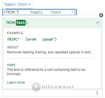
What Is TRIM Function in Google Sheets?
The TRIM function in Google Sheets removes leading, trailing, and repeated spaces.
Syntax
The syntax of TRIM function is as follows:
Argument
| Argument | Requirement | Function |
|---|---|---|
| Text | Required | Reference or text containing the text to be trimmed |
Output
The formula TRIM (“ Supply Chain ”) will show Supply Chain as output.
4 Easy Examples of Using TRIM Function in Google Sheets
Here, we’ll demonstrate 4 easy examples of how to use the TRIM function in Google Sheets. The TRIM function will also be combined with other functions like the ARRAYFORMULA, SPLIT, and FLATTEN functions for advanced operations. Now, let’s go through the methods.
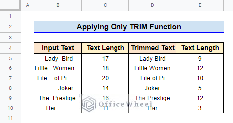
1. Applying Only TRIM Function
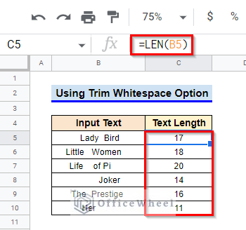
First, let’s get used to our datasheet for this method. The datasheet consists of several input texts with additional leading, trailing, and repeated spaces. The text lengths are also shown using the LEN function. We will use the TRIM function to remove the additional spaces.
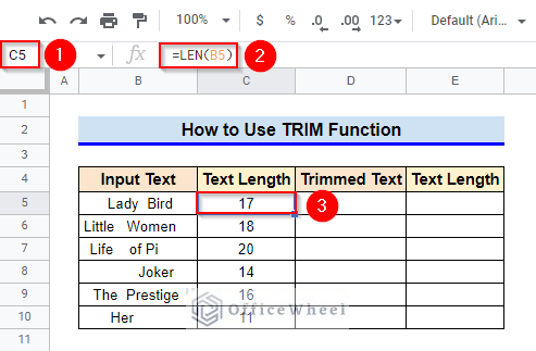
1.1 Input Direct Text Value
We can input direct text values as the argument for the TRIM function.
Steps:
- First, select Cell D5 and type in the following formula and then press the Enter key-
=TRIM(" Lady Bird ")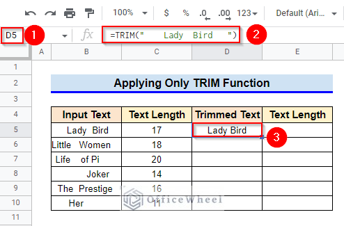
- To check whether the function has actually worked as required, select Cell E5 and type in the following formula. After that, press Enter As you can see, the text length has changed from 17 to 9.
=LEN(D5)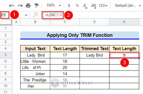
- Similarly, perform the trim operations in other cells of Column D and check the trimmed text length using the LEN function.
1.2 Enter Cell Reference
Using direct text values as an argument can be tedious for large texts or large datasets. An alternative is to use cell references instead.
Steps:
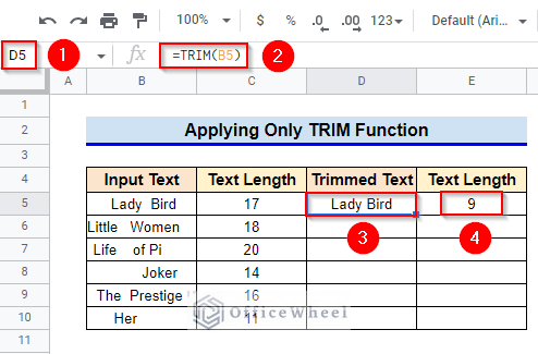
- Select Cell D5 and then type in the following formula. Then, press the Enter key to see the trimmed text.
=TRIM(B5)- Use the LEN function as described previously to check the length of the text after trimming.
- Now, select Cell D5 and use the Fill Handle icon to copy the formula into other cells of Column D.
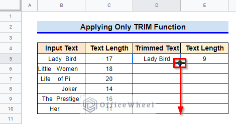
- Similarly, use Fill Handle to copy the formula in Cell E5 to other cells of Column E.

Read More: How to Fill Down an Entire Column in Google Sheets (4 Easy Ways)
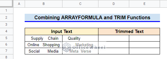
2. Combining ARRAYFORMULA and TRIM Functions
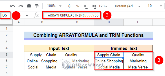
We can apply a combination of the ARRAYFORMULA function and the TRIM function to remove additional spaces from the texts of an array. It will save time because it will return all the output directly as an array. For that, we have taken the following dataset.
Steps:
- First, select Cell D5 and then type in the following formula. After that, press the Enter key to see the output.
=ARRAYFORMULA(TRIM(B5:C7))Now see, we got all the output at a time.
Formula Breakdown
- TRIM(B5:C7)
First, the TRIM function removes the leading, trailing, or repeated spaces for every text value of the array B5:C7.
- ARRAYFORMULA(TRIM(B5:C7))
After that, the ARRAYFORMULA function will help to display the trimmed array.
Read More: How to Use ARRAYFORMULA with IF Function in Google Sheets
Similar Readings
- How to Format Date with Formula in Google Sheets (3 Easy Ways)
- Use the DATEVALUE Function in Google Sheets (An Easy Guide)
- How to Compare Text in Google Sheets (3 Easy Ways)
- Use RIGHT Function in Google Sheets (6 Suitable Examples)
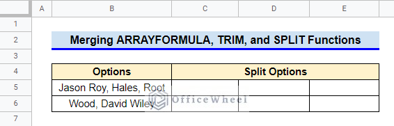
3. Merging ARRAYFORMULA, TRIM, and SPLIT Functions
We often use the SPLIT function for splitting multiple options from a single cell to multiple cells in a row. But the leading space used between the options of a single cell remains. Therefore, we can merge the ARRAYFORMULA and TRIM functions with the SPLIT function to remove these leading spaces. The dataset for this method is as follows:
Steps:
- First, select Cell C5 and then type in the following formula. Finally, press the Enter key to see the output.
=ARRAYFORMULA(TRIM(SPLIT(B5:B6,“,”)))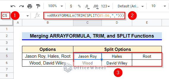
Formula Breakdown
- SPLIT(B5:B6,“,”)
At the beginning of execution, the SPLIT function will divide the input texts from a cell into fragments around the Comma (,) symbol and then puts them in cells of a row.
- TRIM(SPLIT(B5:B6,“,”)
After that, the TRIM function removes additional leading space from each fragmented text returned by the SPLIT function.
- ARRAYFORMULA(TRIM(SPLIT(B5:B6,“,”)))
In the end, the ARRAYFORMULA function helps with displaying the array.
Read More: How to Merge Columns in Google Sheets
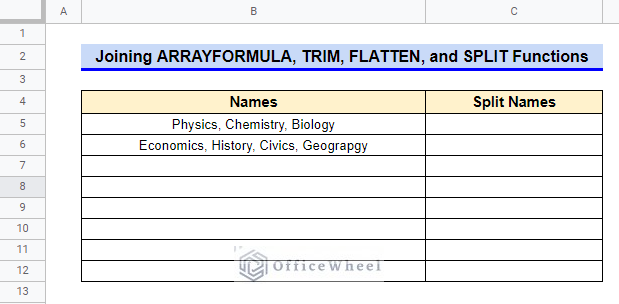
4. Joining ARRAYFORMULA, TRIM, FLATTEN and SPLIT Functions
We can show the output of method 3 in a single column by joining the FLATTEN function with the previously used ARRAYFORMULA, TRIM, and SPLIT functions. Here is the dataset required for this method.
Steps:
- First, select Cell C5 and then type in the following formula. After that press Enter key to view the output-
=ARRAYFORMULA(TRIM(FLATTEN(SPLIT(B5:B6,“,”))))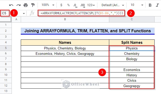
Formula Breakdown
- SPLIT(B5:B6,“,”)
First, the SPLIT function divides the texts in array B5:B6 around the Comma (,) symbol and then puts them in different cells in a row.
- FLATTEN(SPLIT(B5:B6,“,”))
Then, the FLATTEN function puts the values returned by the SPLIT function into a column.
- TRIM(FLATTEN(SPLIT(B5:B6,“,”)))
After that, the TRIM function removes the leading spaces from the text values.
- ARRAYFORMULA(TRIM(FLATTEN(SPLIT(B5:B6,“,”))))
Finally, the ARRAYFORMULA function helps with displaying the output array.
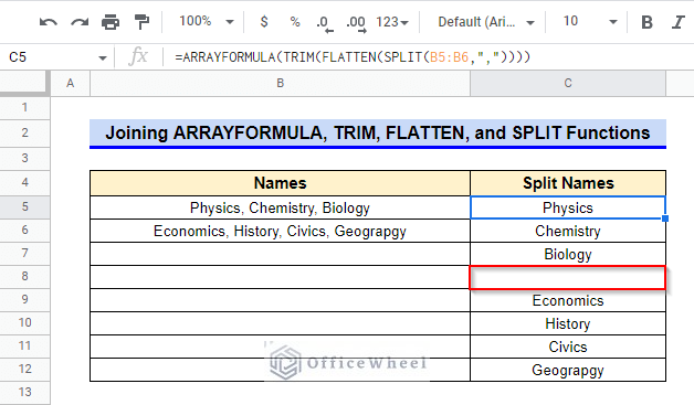
- Here, Cell B5 has 3 values, whereas Cell B6 has 4 values. The FLATTEN function takes the maximum value of 4 and shows the values as a set of 4 entries in a column. That’s why Cell C8 is empty.
Read More: How to Link Cells Between Tabs in Google Sheets (2 Examples)
Alternate of TRIM Function in Google Sheets
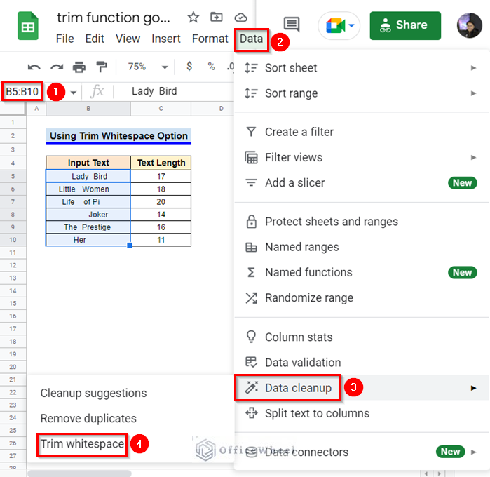
An alternative to using the TRIM function is to use the Trim Whitespace option from the Data ribbon. We’ll be using the following dataset for this alternate method.
Steps:
- First, select the array B5:B10 and then go to the Data ribbon. Then from the Data Cleanup option, click on Trim Whitespace.
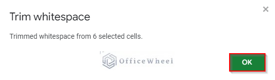
- A window like the following will pop out. Click on OK.
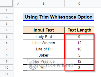
- The additional spaces in selected cells have now been removed and it is also evident from the change in text length.
Conclusion
This ends our article on learning how to use the TRIM function in Google Sheets. I hope the demonstrated methods and examples will satisfy your requirements. Feel free to leave your thoughts on the article in the comment box.
Related Articles
- How to Use IF and OR Formula in Google Sheets (2 Examples)
- Google Sheets: How to Autofill Based on Another Field (4 Easy Ways)
- How to VLOOKUP Last Match in Google Sheets (5 Simple Ways)
- 2 Helpful Examples to VLOOKUP by Date in Google Sheets
- How to Ignore 0 for Standard Deviation Formula in Google Sheets
- Multi Row Dynamic Dependent Drop Down List in Google Sheets
- How to Create Dependent Drop Down List in Google Sheets
- Highlight Duplicates for Multiple Columns in Google Sheets