In Google Sheets, the easiest way to remove duplicates from a vast range of data is using the Filter menu. With the help of the filter menu just select the duplicates, right-click, and delete. In this article, we will explain how to use a filter in Google Sheets to remove duplicates in a column.
A Sample of Practice Spreadsheet
You can download spreadsheets from here and practice.
3 Suitable Ways to Use Filter to Remove Duplicates in Column in Google Sheets
You should consider the word Duplicate in Google Sheets in a broader sense because it mostly depends on the data formatting in the sheet. We use two datasets to show the three methods of Filtering duplicates.
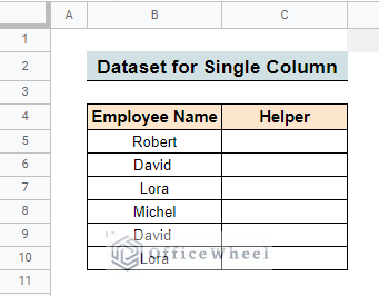
We will use a dataset containing Employee Name to filter and remove the duplicates from a single column of data.
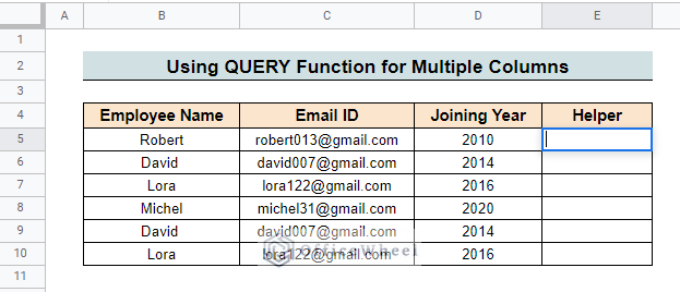
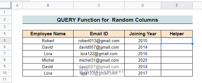
For showing multiple and random columns method, we create a dataset containing three columns: Employee Name, Email ID, and Joining Year.
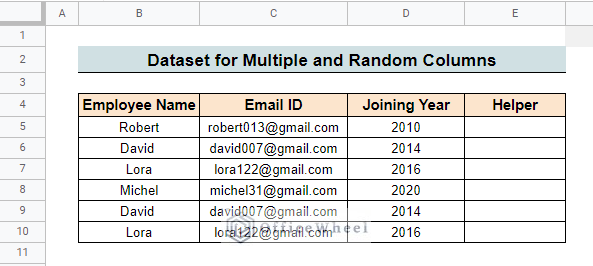
In both datasets, the Helper column will be used to filter the dataset.
Tip: You can hide the Helper column in your worksheet after you are done using it.
1. For Single Column
We can use three different functions for a single column to filter Google Sheets to remove duplicates in a column. The formulas and their use in filtering data are described below:
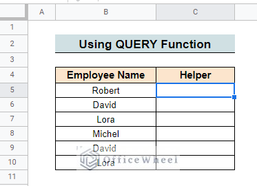
1.1 Using QUERY Function
Through the QUERY function, you can filter your data in any format you want. It will help you to reach your data of interest from a broad dataset. To apply the method,
Steps:
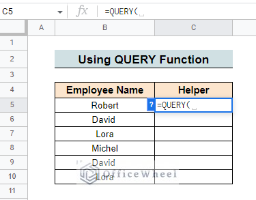
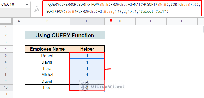
- First, select a cell to insert the function. Here we are going to apply it in cell C5 in the Helper column.
- Open the QUERY function in cell C5.
- Now, we will create a compound formula taking the help of ROW, SORT, and MATCH functions to state the range and duplicate conditions of the QUERY. (The formula breakdown is presented below)
=QUERY(IFERROR(SORT({ROW(B5:B)-ROW(B5)+2-MATCH(SORT(B5:B),SORT(B5:B),0),SORT(ROW(B5:B)+2-ROW(B5)+2,B5:B,1)},2,1),),"Select Col1")-
Press ENTER to apply the formula and you will find the results in the Helper column. It shows the count of the Names as they occur.
Formula Breakdown
- MATCH(SORT(B5:B),SORT(B5:B),0): Here, SORT(B5:B) sorts the values in column B starting from cell B5. The MATCH function uses the output of the SORT function to return the position of matching values.
- SORT(ROW(B5:B)+2-ROW(B5)+2,B5:B,1): ROW(B5:B) and ROW(B5) returns the respective row numbers. Then the SORT function sorts the values from B5 to the entire B column and marks them by adding 1 for each value.
- SORT({ROW(B5:B)-ROW(B5)+2-MATCH(SORT(B5:B),SORT(B5:B),0),SORT(ROW(B5:B)+2-ROW(B5)+2,B5:B,1)},2,1): Here the curly brackets {} converts all of the outputs to an array. Then the SORT function sorts the outputs and returns 1 for the unique values and 2 for duplicates.
- IFERROR(…): The IFERROR function returns an empty string in case of errors. Otherwise, it returns the formula output.
- QUERY(…,”Select Col1″): This is the actual query action. It queries the values in Column B (which is the first column of the selected range) to find the duplicates.
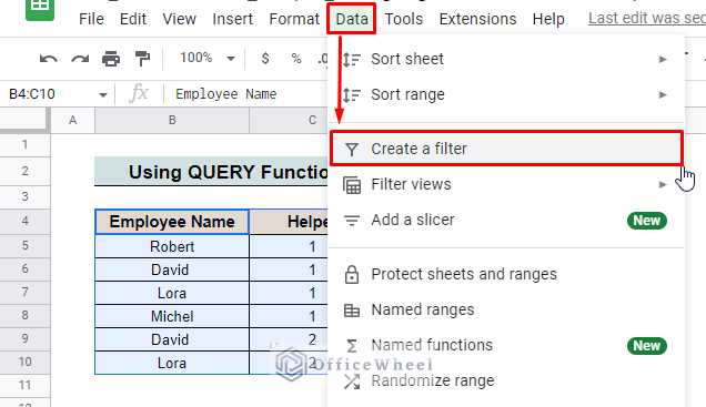
- Next, select the entire table.
- Go to Data and select Create a filter.
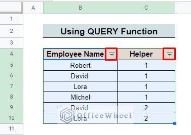
- You can find the filter sign beside the column title.
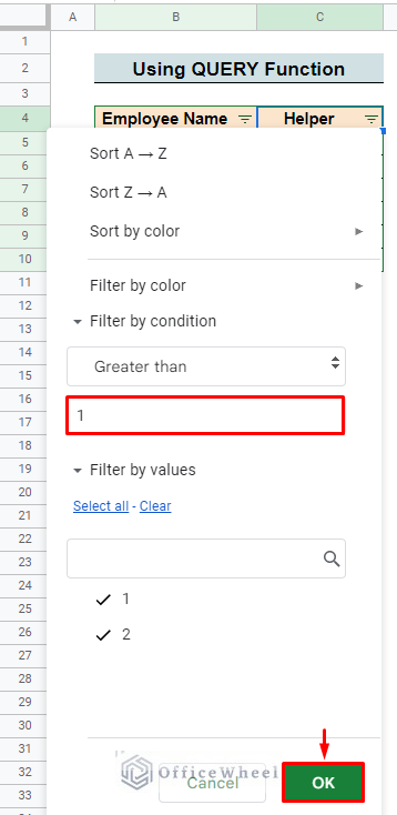
- Go to the Helper column’s filter bar and select the Filter by condition bar. Now click on the Greater than option bar.
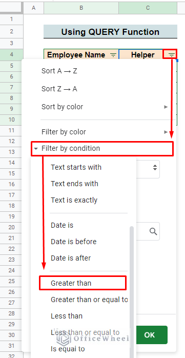
- Now insert 1 in the box and press OK to operate.
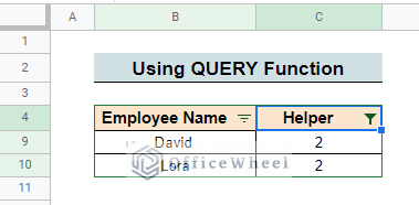
- Finally, you can find the duplicate filter value in the dataset. You can remove all of them by clicking the DELETE option.
1.2 Applying ARRAYFORMULA Function
The ARRAYFORMULA function is used to represent a huge range of data instead of a single value. In this article, we use this formula to filter the column or columns. To apply this formula,
Steps:
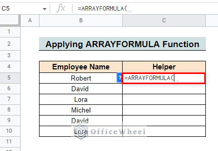
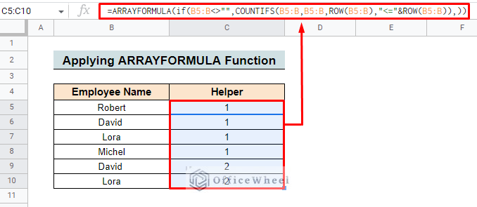
- First, select cell C5 in the Helper column and insert the ARRAYFORMULA function.
=ARRAYFORMULA(IF(B5:B<>"",COUNTIFS(B5:B,B5:B,ROW(B5:B),"<="&ROW(B5:B)),))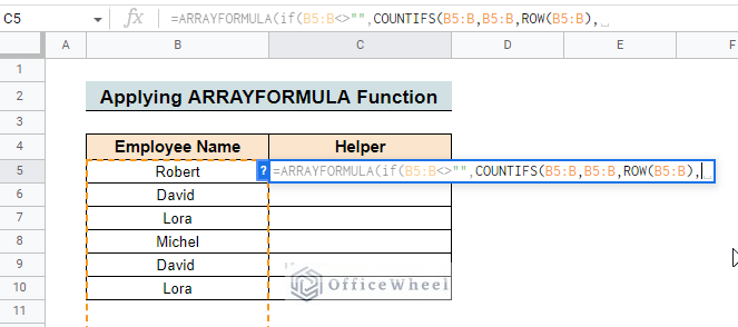
- Here is the resulting Helper Column:
Formula Breakdown
- COUNTIFS(B5:B, B5:B, ROW(B5:B), “<=”&ROW(B5:B)): The COUNTIFS function will evaluate two criteria in two ranges. Firstly, it will look for the value in the B5 cell in the B5:B range. Secondly, it will evaluate if the ROW(B5:B) or the row number of the B5 cell is less than or equal to the row number returned by ROW(B5:B). If the cell value fulfills both conditions, then it will count the value. In this case, it will return 1.
- IF(B5:B<>””,COUNTIFS(B5:B,B5:B,ROW(B5:B),”<=”&ROW(B5:B)),): This is just a normal IF formula. The formula becomes if(B5:B<>””,1,). So, if the value in the B5 cell is not equal to zero then the formula will return 1. Here, we have added the ARRAYFORMULA around the IF function just to make the formula more adaptable and get the output values as an array.
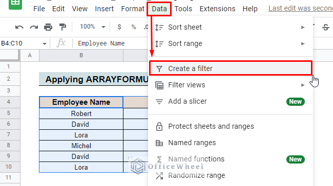
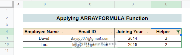
- Then go to Data and select Create a filter.
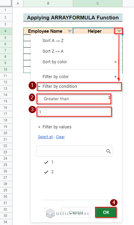
- After that, select Filter by condition > Greater than > 1. Finally, press OK.
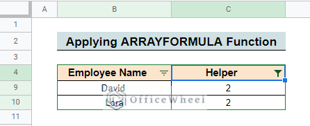
- You can find the filtered duplicate values in your dataset. Now you can delete them easily.
Read More: How to Use ARRAYFORMULA in Google Sheets (6 Examples)
1.3 Inserting IF and COUNTIF Functions
In Google Sheets, the IF and COUNTIF function are used to solve the different conditions. These functions combinedly filter duplicates from Google Sheets.
Steps:
- Select cell C5 and insert the formula there.
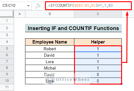
=IF(COUNTIF($B$5:B5,B5)=1,1,0)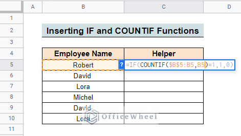
Formula Breakdown
- COUNTIF($B$5:B5, B5): The COUNTIF function will evaluate two criteria in two ranges. Firstly, it will look for the value in the $B$5 cell. Secondly, it will evaluate if the row number of the B5 cell is less than or equal to the row number returned by B5. If the cell value fulfills both conditions, then it will count the value. In this case, it will return 1.
- IF(COUNTIF($B$5:B5,B5)=1,1,0): This is just a normal IF formula. So, if the value in the B5 cell is not equal to 0 then the formula will return 1.
- Copy the formula down the entire column by using the fill handle.
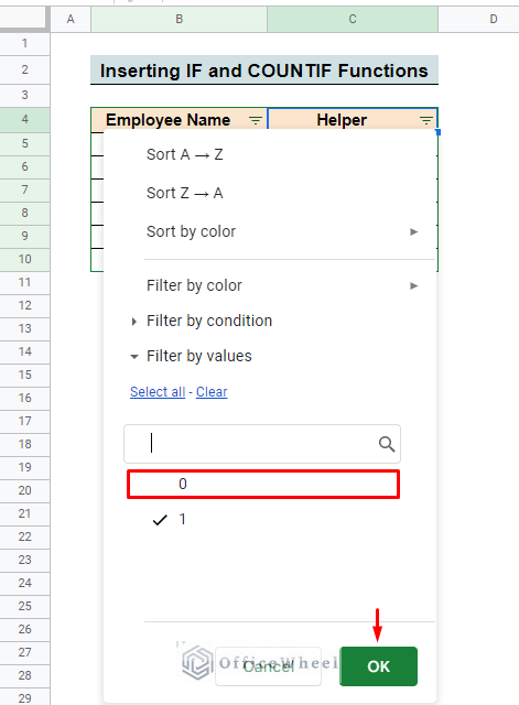
- Select the entire dataset and go to menu bar, then select Data > Create a filter to add a filter option in your columns.
- Then remove the tick mark from the 0. So that you can filter only those values containing 1.
- Finally, press OK to apply.
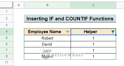
- You can find only the filtered unique values in the dataset.
Read More: How to Use Formula to Highlight Duplicates in Google Sheets
Similar Readings
- How to Sum Using ARRAYFORMULA in Google Sheets
- VLOOKUP Last Match in Google Sheets (5 Simple Ways)
- How to Calculate Weighted Average Using IF Function in Google Sheets
- Format Date with Formula in Google Sheets (3 Easy Ways)
- How to Use the Find Function in Google Sheets (An Easy Guide)
2. For Multiple Columns
You can also use the same functions to filter duplicates from multiple columns in Google Sheets. To do so here we create a dataset of three columns.
2.1 Using the QUERY Function
The QUERY function method remains the same as applied to the single column. For multiple columns,
Steps:
- Select the cell to insert the QUERY function. Here, we select cell E5 in the Helper column.
- The QUERY formula for multiple columns is:
=QUERY({B5:B,IFERROR(SORT({ROW(B5:B)-ROW(B5)+2-MATCH(SORT(B5:B&C5:C&D5:D),SORT(B5:B&C5:C&D5:D),0),SORT(ROW(B5:B)+2-ROW(B5)+2,B5:B&C5:C&D5:D,1)},2,1),)},"Select Col2 where Col1 is not null")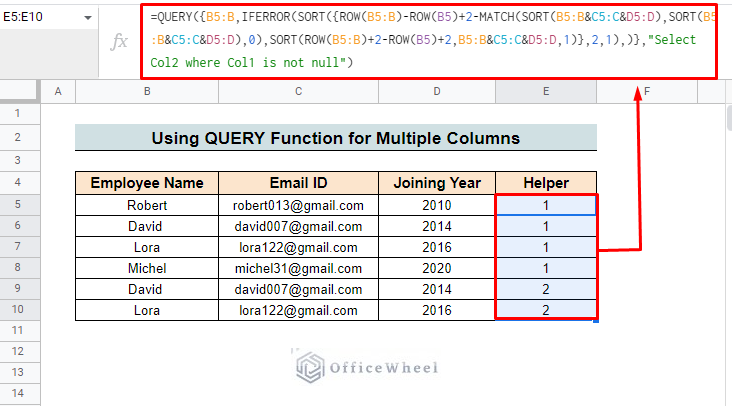
Formula Breakdown
- MATCH(SORT(B5:B&C5:C&D5:D),SORT(B5:B&C5:C&D5:D),0): Here, SORT(B5:B&C5:C&D5:D) sorts the values for the entire table containing columns B, C & D. The MATCH function uses the output of the SORT function to return the position of matching values.
- SORT(ROW(B5:B)+2-ROW(B5)+2,B5:B&C5:C&D5:D,1): ROW(B5:B) and ROW(B5) returns the respective row numbers. Then the SORT function sorts the values from B5, C5 & D5 to the entire B, C & D column and marks them by adding 1 for each value.
- SORT({ROW(B5:B)-ROW(B5)+2-MATCH(SORT(B5:B&C5:C&D5:D),SORT(B5:B&C5:C&D5:D),0),SORT(ROW(B5:B)+2-ROW(B5)+2,B5:B&C5:C&D5:D,1)},2,1),)}: Here the curly brackets {} converts all of the outputs to an array. Then the SORT function sorts the outputs and returns 1 for the unique values and 2 for duplicates.
- IFERROR(…}: The IFERROR function returns an empty string in case of errors. Otherwise, it returns the formula output.
- QUERY({B5:B,…,”Select Col2 where Col1 is not null”): It queries the values in Column B to find the duplicates. “Select Col2 where Col1 is not null” is applicable for multiple columns.
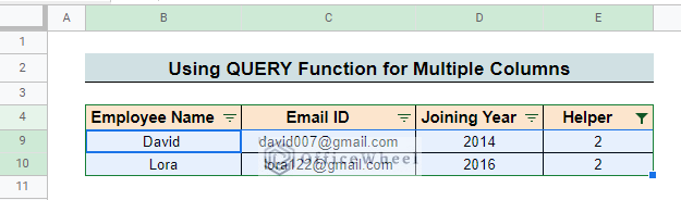
- Then go to the Data and select Create a filter.
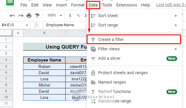
- The filter symbol is added just beside the column title.
- Now, go to the filter option, select Filter by condition, then choose Greater than and enter 1 in the box below.
- Finally, press OK.
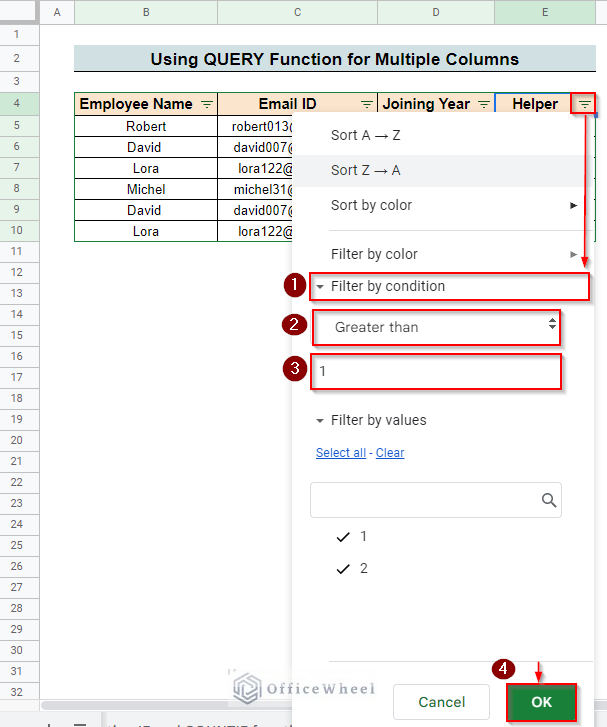
- You can find duplicate values in the dataset. You can remove them by using the Delete option.
Read More: How to Find and Remove Duplicates in Google Sheets (5 Ways)
2.2 Applying ARRAYFORMULA Function
The ARRAYFORMULA function is also the same for multiple columns. There is a small difference only in cell selection. So, to apply the ARRAYFORMULA function for multiple columns.
Steps:
- First, select the cell and enter the ARRAYFORMULA function. Here, we insert the formula into the Helper column.
=ARRAYFORMULA(IF(B5:B<>"",COUNTIFS(B5:B&C5:C&D5:D,B5:B&C5:C&D5:D,ROW(B5:B),"<="&ROW(B5:B)),))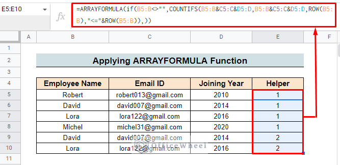
Formula Breakdown
- COUNTIFS(B5:B&C5:C&D5:D,B5:B&C5:C&D5:D,ROW(B5:B),”<=”&ROW(B5:B)): The COUNTIFS function will evaluate two criteria in two ranges. Firstly, it will look for the value in the B5:B&C5:C&D5:D ranges. Secondly, it will evaluate if the ROW(B5:B) or the row number of the B5 cell is less than or equal to the row number returned by ROW(B5:B). If the cell value fulfills both conditions then it will count the value. In this case, it will return 1.
- IF(B5:B<>””,COUNTIFS(B5:B&C5:C&D5:D,B5:B&C5:C&D5:D,ROW(B5:B),”<=”&ROW(B5:B)),): This is just a normal IF formula. The formula becomes IF(B5:B<>””,1,). So, if the value in the B5 cell is not equal to zero then the formula will return 1. Here, we have added the ARRAYFORMULA around the IF function just to make the formula more adaptable and get the output values as an array.
- Then, ‘Select’ Filter by condition > Greater than > 1 > OK.

- Now you can easily find the duplicates and can remove them if necessary.
Read More: How to Highlight Duplicates for Multiple Columns in Google Sheets
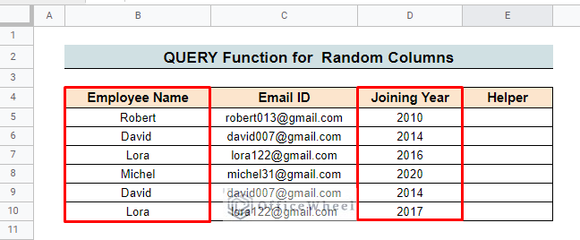
3. For Random Columns
You can use the QUERY and ARRAYFORMULA functions for filtering random columns in Google Sheets. The formula structure is the same as the multiple-column formulas. The main changes are in the column range selection. For multiple columns, you can select all the columns to apply the filter, but for the random column, you have to choose the specific columns from where you want to filter your data. Here, we select B and D columns for applying the methods.
3.1 QUERY Function for Random Columns
- First, we select the E5 cell in the Helper column.
- Enter the QUERY formula in the selected cell.
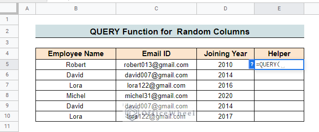
- The QUERY function for random columns is:
=QUERY({B5:B,IFERROR(SORT({ROW(B5:B)-ROW(B5)+2-MATCH(SORT(B5:B&D5:D),SORT(B5:B&D5:D),0),SORT(ROW(B5:B)+2-ROW(B5)+2,B5:B&D5:D,1)},2,1),)},"Select Col2 where Col1 is not null")Formula Breakdown
- MATCH(SORT(B5:B&D5:D),SORT(B5:B&D5:D),0): Here, SORT(B5:B&D5:D) sorts the values for the entire table containing columns B & D. The MATCH function uses the output of the SORT function to return the position of matching values.
- SORT(ROW(B5:B)+2-ROW(B5)+2,B5:B&D5:D,1): ROW(B5:B) and ROW(B5) returns the respective row numbers. Then the SORT function sorts the values from B5 & D5 to the entire B & D column and marks them by adding 1 for each value.
- SORT({ROW(B5:B)-ROW(B5)+2-MATCH(SORT(B5:B&D5:D),SORT(B5:B&D5:D),0),SORT(ROW(B5:B)+2-ROW(B5)+2,B5:B&D5:D,1)},2,1),)}: Here the curly brackets {} converts all of the outputs to an array. Then the SORT function sorts the outputs and returns 1 for the unique values and 2 for duplicates.
- IFERROR(…)}: The IFERROR function returns an empty string in case of errors. Otherwise, it returns the formula output.
- QUERY({B5:B,…,”Select Col2 where Col1 is not null”): It queries the values in Column B to find the duplicates. “Select Col2 where Col1 is not null” is applicable for multiple columns or random columns.
- Here, I just exclude column C from the function. As I want to find the duplicates from Employment Name and Joining Year columns.
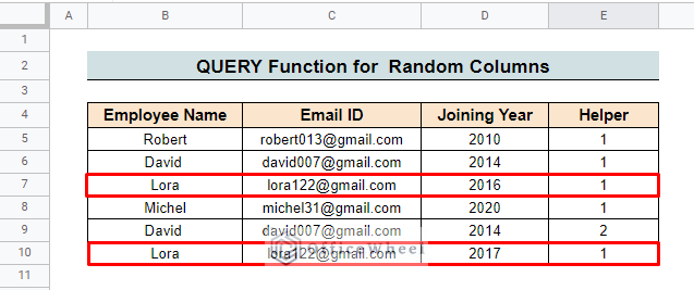
- Here, Though the Employee Name and Email ID of these two employees are the same, they do not make duplicates because the Joining Year is different. We select B and D columns as our random data to filter so, the C column is not under consideration.
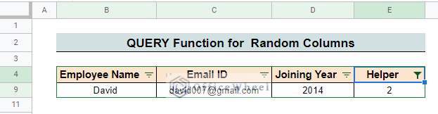
- You can see the final result in the dataset.
Read More: Highlight Duplicates in Google Sheets (4 Ways)
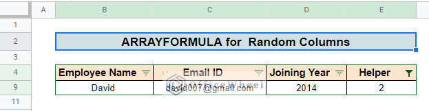
3.2 ARRAYFORMULA Function for Random Columns
For random columns, the ARRAYFORMULA function will help you to filter a range of duplicates. We select E5 cell to apply the method.

- Here, we use the formula in cell E5 and go through the same process as multiple columns.
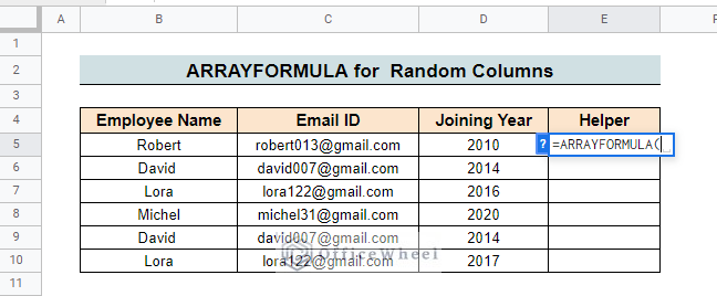
- The ARRAYFORMULA function for the random column is:
=ARRAYFORMULA(IF(B5:B<>"",COUNTIFS(B5:B&D5:D,B5:B&D5:D,ROW(B5:B),"<="&ROW(B5:B)),))Formula Breakdown
- COUNTIFS(B5:B&D5:D,B5:B&D5:D,ROW(B5:B),”<=”&ROW(B5:B)): The COUNTIFS function will evaluate two criteria in two ranges. Firstly, it will look for the value in the B5:B&D5:D ranges. Secondly, it will evaluate if the ROW(B5:B) or the row number of the B5 cell is less than or equal to the row number returned by ROW(B5:B). If the cell value fulfills the condition then it will count the value. In this case, it will return 1.
- IF(B5:B<>””,COUNTIFS(B5:B&D5:D,B5:B&D5:D,ROW(B5:B),”<=”&ROW(B5:B)),): This is just a normal IF formula. The formula becomes IF(B5:B<>””,1,). So, if the value in the B5 cell is not equal to zero then the formula will return 1. Here, we have added the ARRAYFORMULA around the IF function just to make the formula more adaptable and get the output values as an array.
- Another process is the same as we discussed before. Here, we present the final outcome for this specific formula.
Things to Remember
- You have to insert the function carefully.
- The column range must be input properly in every function.
- You should be careful about symbols in functions.
Conclusion
After going through this article, we hope now you can easily understand how to use the filter in Google Sheets to remove duplicates in a column. For exploring more techniques in Google Sheets, you can also visit our OfficeWheel website.
Related Articles
- How to Remove Duplicates in Google Sheets Without Shifting Cells
- Remove Duplicates in Column on Different Sheets in Google Sheets
- How to Remove Both Duplicates in Google Sheets (2 Easy Ways)
- Count Duplicates In Google Sheets (3 Ways)
- How to Remove Duplicates in Google Sheets Using Formula
- Create Dependent Drop Down List in Google Sheets
- How to Link Cells Between Tabs in Google Sheets (2 Examples)