While there are no direct ways, it is still possible to find the top 10 values in a Google Sheets pivot table.
In this article, we will explain the limitations and look at some indirect ways to filter out the top values using the many tools that Google Sheets has for us.
Let’s get started.
Can you find the top 10 values in a Google Sheets Pivot Table?
No. While there are multiple easy ways to filter the top 10 values from a regular dataset in Google Sheets, there are no direct ways to do so from the Pivot table editor.
This is a disadvantage of Google Sheets considering that this can be easily done in Excel. Hopefully, a future update will fix this. There is a multitude of other advantages of the pivot table editor, but today’s discussion does not focus on those.
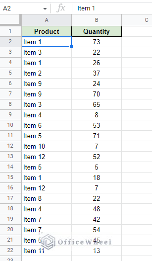
Back to the topic at hand, here we have a sample dataset that we will use to create a pivot table:
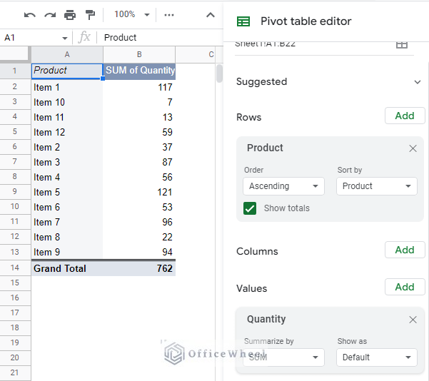
The resultant pivot table:
Now, if we want to find the top values, all we have to do is sort the Google Sheets pivot table using the following conditions:
- Rows > Product
- Order: Descending
- Sort by: SUM of Quantity
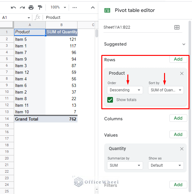
However, this is the limit of what we can do.
While we have sorted the table to show the top values, all the values will be presented. There is no way to filter the top 10 values from the pivot table editor.
But that doesn’t mean that it is impossible.
We have a couple of indirect ways to filter the top 10 values in a pivot using certain functions of Google Sheets.
Let’s have a look.
Indirect Ways to Show the Top 10 Values in a Google Sheets Pivot Table
1. Take the Help of the QUERY function to Filter the Top 10 Values
If we can’t directly filter the top 10 values in a pivot table, let’s bring the top 10 values to the pivot table instead.
It is a brute force method, but it satisfies the conditions.
This process rests on the back of the QUERY function.
QUERY(data, query, [headers])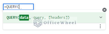
The idea is to create a top 10 filter using the QUERY function and then use the result to create a pivot table.
Step 1: In the same worksheet as the source data, open the QUERY function beside the dataset.
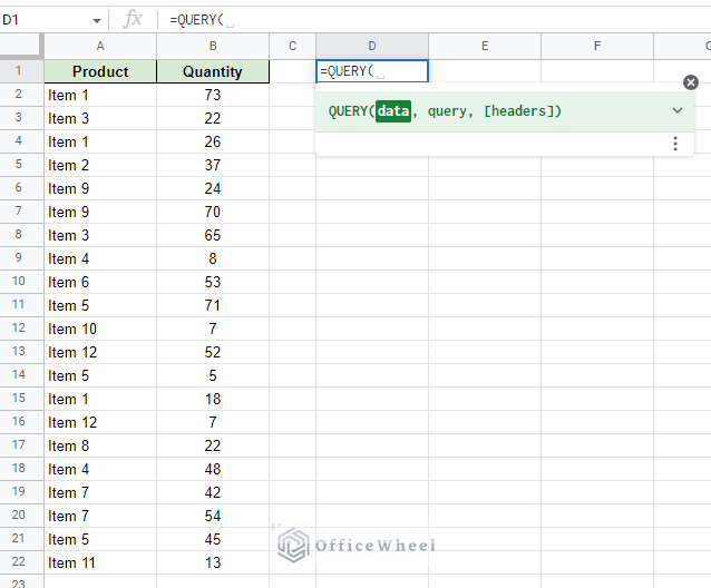
Step 2: Apply the following QUERY formula:
=QUERY({A1:B22},"Select Col1,Sum(Col2) group by Col1 order by Sum(Col2) desc")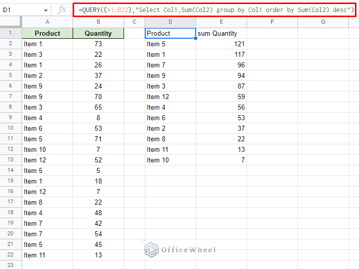
What we have just created is the same sorted pivot table we have just seen in the previous section. It contains all the values grouped and in descending order.
Step 3: What we need now is to filter only the top 10 values. Simply add the “limit 10” condition at the end of the QUERY.
=QUERY({A1:B22},"Select Col1,Sum(Col2) group by Col1 order by Sum(Col2) desc limit 10")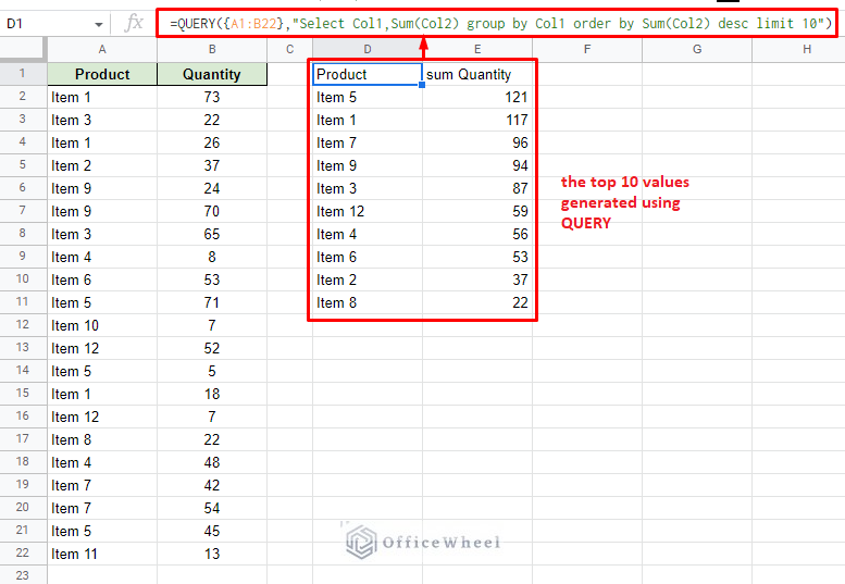
Step 4: Create a new pivot table with this new table generated with QUERY.
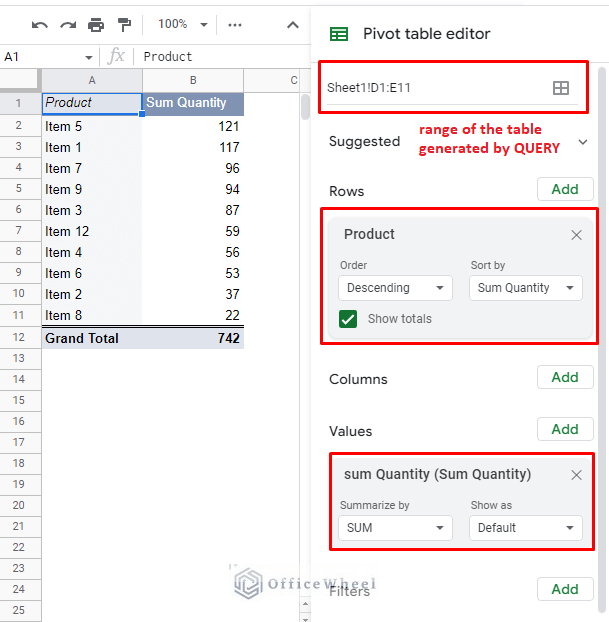
Since this pivot table takes its values directly from the QUERY table from the main worksheet, any changes made to the source dataset will be reflected in this table.
So, if data changes enough to update the top 10 values, the QUERY table will also update itself and subsequently change the pivot table.
2. Use Regular Expressions to Create a Custom Formula to Use as a Filter for the Top 10 Values
We all know that filters are the best way to get any value that we desire, even the top 10 values. However, since the Google Sheets pivot table does not allow a top 10 filter, we have to take an indirect approach. Namely a custom formula for filters.
Learn More: Using Custom Formula in a Google Sheets Pivot Table (3 Easy Ways)
The formula in question is based on the use of regular expressions. The idea is to match the top 10 Item names instead of the Quantity in descending order.
Remember the QUERY formula used to find the top 10 values in the previous section?
=QUERY({A1:B22},"Select Col1,Sum(Col2) group by Col1 order by Sum(Col2) desc limit 10")We will use this formula to piggyback the regular expressions to use as the custom formula in the pivot table.
Step 1: Modify the QUERY formula to only give us the Item names of the top 10 Items.
=QUERY(QUERY({A2:B22},"Select Col1,Sum(Col2) group by Col1 order by Sum(Col2) desc limit 10 label Sum(Col2)''"),"Select Col1")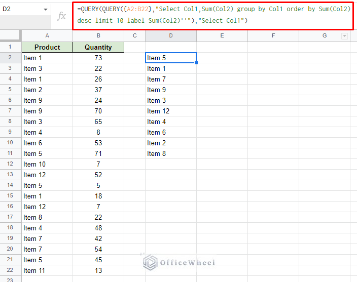
Step 2: Now to set up the regular expression format. The format of Item names to match as a regular expression should be like this:
^Item 5$|^Item 1$|^Item 7$|… and so onSo, to list the Item names as a regular expression:
=ArrayFormula("^"&QUERY(QUERY({A2:B22},"Select Col1,Sum(Col2) group by Col1 order by Sum(Col2) desc limit 10 label Sum(Col2)''"),"Select Col1")&"$")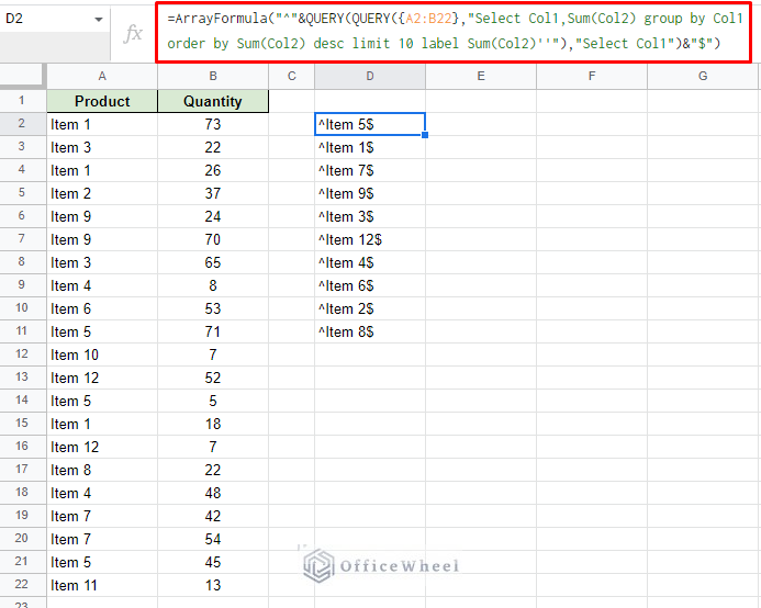
Step 3: As you may have noticed, we have the pipe symbol (|) missing from the column. To add this symbol, we will use the TEXTJOIN function. The updated formula:
=ArrayFormula(TEXTJOIN("|",1,"^"&QUERY(QUERY({A2:B22},"Select Col1,Sum(Col2) group by Col1 order by Sum(Col2) desc limit 10 label Sum(Col2)''"),"Select Col1")&"$"))Step 4: Finally, since we are matching the names with regular expressions, we must use the REGEXMATCH function.
The final formula:
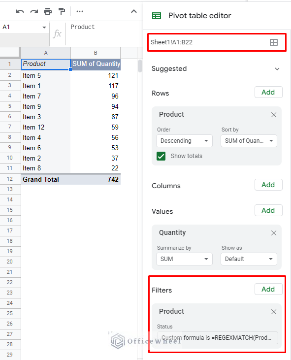
=REGEXMATCH(Product,ArrayFormula(TEXTJOIN("|",1,"^"&QUERY(QUERY({A2:B22},"Select Col1,Sum(Col2) group by Col1 order by Sum(Col2) desc limit 10 label Sum(Col2)''"),"Select Col1")&"$")))Step 5: Apply the custom formula in the Filter of the Google Sheets Pivot table.
Filter > Add > Product > Filter by condition > Custom formula is
To change the number of topmost values, simply change the Query Limit clause from 10 to any other number in the QUERY function.
Final Words
Even though there are no direct ways to filter the top 10 values in the Google Sheets pivot table editor, we have other tools to utilize that will help us do so.
The simplest way is to that advantage of the QUERY function and then later use the results to create a pivot table.
Feel free to leave any queries or advice you might have in the comments section below.
Related Articles for Reading
- How to Apply and Work with a Calculated Field of a Google Sheets Pivot Table
- Pivot Table Formatting in Google Sheets (3 Easy Ways)
- Google Sheets: Create a Pivot Table with Data from Multiple Sheets
- How to Group by Month in a Google Sheets Pivot Table (An Easy Guide)
- Google Sheets Pivot Table: Sort by Value (3 Easy Ways)