Conditional Formatting Highlight Duplicates in Google Sheets

No matter how much we try to avoid it, some duplicates often remain while working with large datasets in Google Sheets. Having duplicate values is annoying and unnecessary. Fortunately, you can easily check for duplicates within datasets in Google Sheets. In this article, we will show how to highlight duplicates using conditional formatting in Google Sheets. So, let’s start.

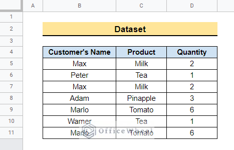
A Sample of Practice Spreadsheet

What Is Conditional Formatting in Google Sheets?

Before we know how to apply conditional formatting to highlight duplicates, let’s learn a little about this feature in Google Sheets.

While working on Google Sheets, your dataset may contain different types of products. Each category may have unique or duplicate values. The Conditional formatting feature in Google Sheets allows us to format and highlight datasets properly based on specific rules or criteria. You can apply the Bold, Italic, Underline, and Strikethrough formats, change font colors, and highlight cells based on criteria using this feature.

4 Examples of Conditional Formatting to Highlight Duplicates in Google Sheets

The dataset below contains some Customer’s Names, Products ordered by them along with the corresponding Quantities. Unfortunately, the dataset contains some duplicates which are not desired at all.  Finding duplicates manually in large datasets can be a very time-consuming and tiring job. In this article, we will show you how to highlight duplicates easily using conditional formatting in Google Sheets.

Follow the methods below to learn how to do that.

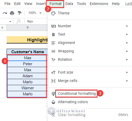
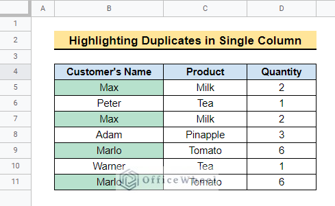
1. Highlight Duplicates in Single Column

Here we will show you how to highlight the duplicate values in a single column using the conditional formatting feature. Follow the steps to see that.

📌 Steps:

• First, select the range B5:B11 and go to Format >> Conditional formatting as shown below.

• Then, the Conditional format rules window will pop up. Next, select the “Custom formula is” option from the Format rules.

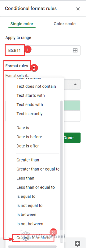
• After that, enter the COUNTIF formula in the Value or formula field and click on Done.

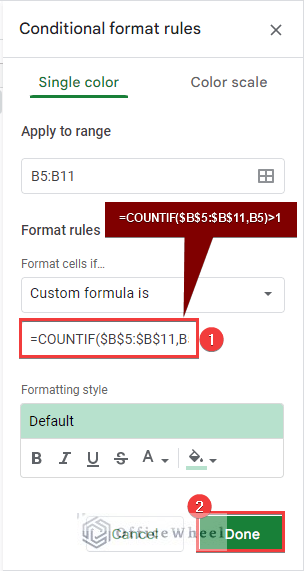
• Here, we have used the COUNTIF function to count the number of appearances of the values in the dataset. If the return value of the function is greater than 1, then the conditional formatting will get activated.
• As a result, the duplicate values will be highlighted with the default color. You can choose different colors using the fill color tool in the Formatting style.

Read More: How to Use Formula to Highlight Duplicates in Google Sheets

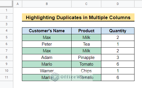
2. Highlight Duplicates in Multiple Columns

We can also highlight duplicate values in multiple columns using conditional formatting. The steps to do that are mentioned below.

📌 Steps:

• First, you need to select the multiple columns where the duplicates are remaining. Here, we will select range B5:C11 instead of B5:B11 in the earlier method. Then go to Format >> Conditional formatting as before.
• After that, select the “Custom Formula is” option from the Format rules in the “Conditional format rules” Next, insert the formula below in the Value or formula box and click Done.

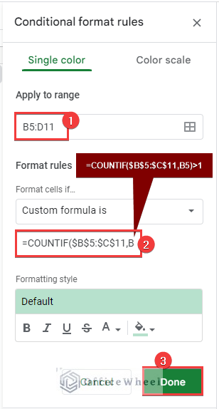
• As a result, the system will highlight the duplicate values as follows.

Read More: Highlight Duplicates in Two Columns in Google Sheets (2 Ways)

3. Highlight Entire Row for Duplicates in Single Column

Now, we will show the way to highlight the entire row for duplicates in a single column. Here we will highlight the rows based on duplicates in the Quantity column. The steps to do that are as follows.

📌 Steps:

• First, select the entire range i.e. the range B5:D11. Then go to Format >> Conditional formatting as earlier.
• Next, apply the following formula for Format rules with the Custom formula. Click on Done after that.

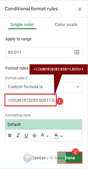
• As a result, the system will highlight all the rows for corresponding duplicates in the Quantity column as follows.

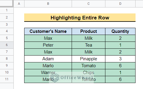
• Here, you must use mixed references in the criteria input of the COUNTIF function. Notice that the column number of the $D5 criteria is fixed but the row number is relative.

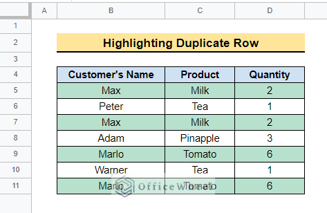
4. Highlight Duplicate Rows

Lastly, we will demonstrate how to highlight duplicate rows. For example, 2 rows will be highlighted if all corresponding values between the rows are the same. The following steps will guide you to do that.

📌 Steps:

• First, select range B5:D11 and go to Format >> Conditional formatting as before. Then go to Format rules >> Format cells if >> Custom formula is in the Conditional format rules window.
• Next, enter the following formula in the Value or formula field and click Done.

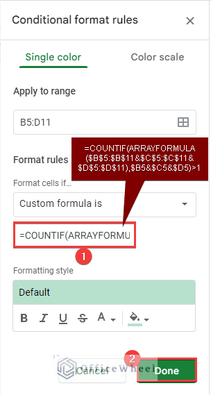
• After inserting the formula, duplicate rows are highlighted as follows.

• Here, the ARRAYFORMULA($B$5:$B$11&$C$5:$C$11&$D$5:$D$11) concatenates the values of each row and creates an array with the concatenated values. For example, it returns MaxMilk2 for the 1st row, PeterTea1 for the 2nd row, and so on. The $B5&$C5&$D5 criteria input for the COUNTIF function does the same.

Things to Remember

• Always lock the data range while inserting the formula. You can press F4 to do that.
• You need to use the mixed references properly in the formulas. Otherwise, you will not get the desired result.

Conclusion

In this article, we have demonstrated 4 practical ways to use conditional formatting to highlight duplicates in Google Sheets. Hopefully, the methods will help you highlight duplicates in your own dataset. Please let us know in the comment section if you have any queries or suggestions. You may also visit our OfficeWheel blog to explore more Google Sheets-related articles.