Suppose you are working on two datasets at the same time. But the dataset is almost similar and there are some data missing in the second dataset. Now, you need to find all the missing data to execute your work. Here, finding all the missing values manually is nearly impossible if the dataset is large. If you try to complete this task manually it will turn into a very time-consuming activity. So, you can find the missing values using formulas quickly and easily. In this article, we will learn how to find missing values between two columns in google sheets.
The overview of this article is above. You can learn more to find missing values if you go through the whole article. So, let’s start.
A Sample of Practice Spreadsheet
You may copy the spreadsheet below and practice by yourself.
2 Suitable Ways to Find Missing Values Between Two Columns in Google Sheets
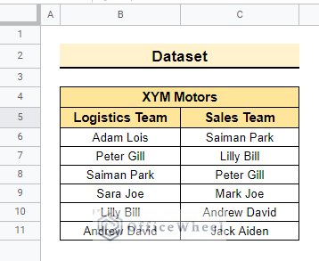
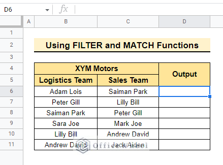
The dataset below contains the employee name of Logistics Team and Sales Team of XYM Motors. Here, we will find the employees who are in the logistics team but missing in the sales team using different functions.
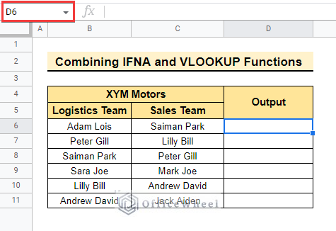
1. Combining IFNA and VLOOKUP Functions
Now, we will find the missing values using The IFNA Function and The VLOOKUP Function combinedly.
📌 Steps:
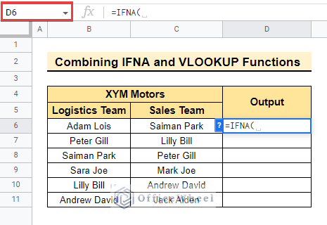
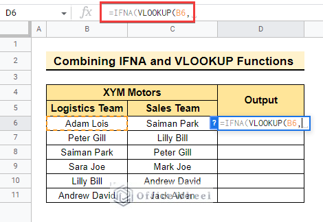
- First, select cell D6 to enter the formulas.
- Now enter the IFNA function to get the desired decision if the value is missing.
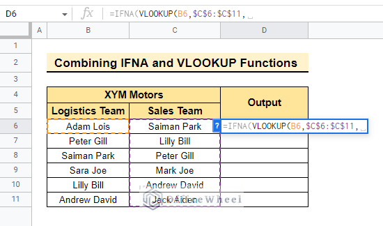
- Then, enter the VLOOKUP function to get the common values in both teams. and select cell B6 as lookup value.
- Here, select the lookup range C6:C11 and lock the range to get the accurate value.
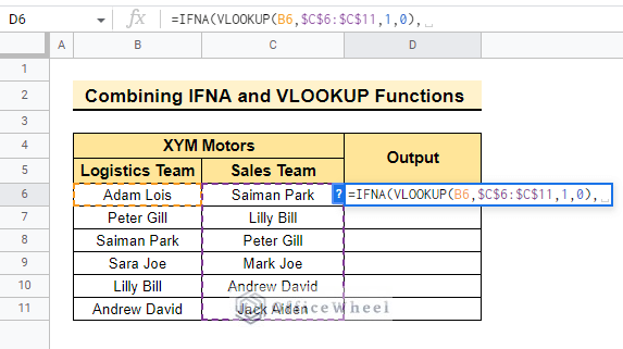
- Consequently, Manually write 1 to get the common value from the first column of the range and terminate the function with 0 or FALSE to get the exact value.
- After completing the VLOOKUP function complete the IFNA function keeping space in double quotes. So that, if the function does not find any common value it returns a blank space as output.
=IFNA(VLOOKUP(B6,$C$6:$C$11,1,0),"")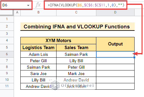
- The function shows the common value and shows blank cells if the value is missing. Here, Adam Lois is missing from the sales team that’s why the output is a blank cell here.
- In the end, drag down the fill handle or double-tap the fill handle to copy the same formula in every cell.
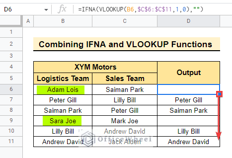
- In this picture, Adam Lois and Sara Joe are highlighted because this two are missing values and are shown as blank cells in the output.
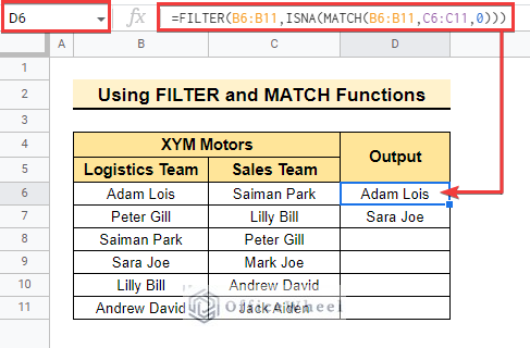
2. Using FILTER and MATCH Functions
Now, we will use the FILTER function and the MATCH function to get the missing values in google sheets using the previous dataset.
📌 Steps:
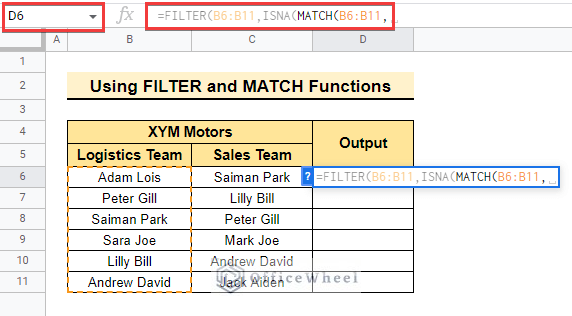
- Initially, select cell D6 to enter the functions.
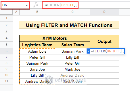
- Therefore, enter the FILTER function to filter the data which is common in both teams and select the lookup range as below.
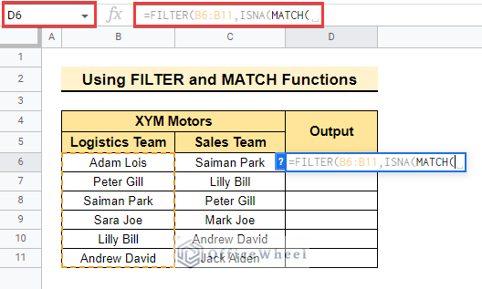
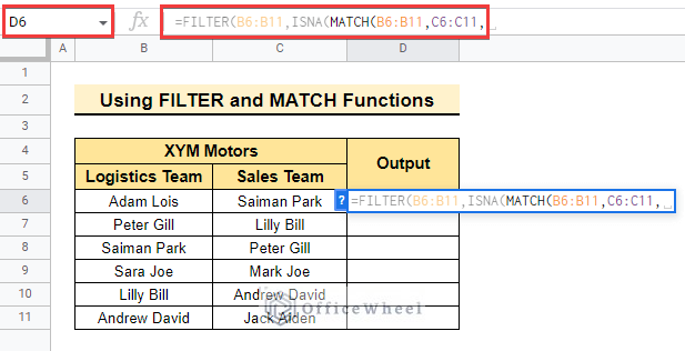
- Now, enter the MATCH function to find the matched values in both teams.
- Moreover, select the lookup range B6:B11 so that the function returns value from lookup range.
- Now, select the result range C6:C11 so that the function searches common values from the result range.
- Finally, write 0 to complete the formula and get the final output as below.
=FILTER(B6:B11,ISNA(MATCH(B6:B11,C6:C11,0)))
Here, the final output represents the missing name of employees who belongs to the logistics team only.
Read More: How to Find Unique Values Between 2 Columns in Google Sheets
Similar Readings
- How to Filter Between Two Dates in Google Sheets
- Difference Between COUNT and COUNTA in Google Sheets
- How to Link Cells Between Tabs in Google Sheets (2 Examples)
- Google Sheets Count Cells Between Two Numbers with COUNTIF Function
- How to Move Between Tabs in Google Sheets (3 Easy Ways)
How to Check If Values Are Missing Between Two Columns in Google Sheets
Here, we will get decisions if the values in the dataset are missing or if they belong to the dataset using different formulas. Here we will use the same dataset we used before.
1. Merging IF and COUNTIF Functions
Moreover, we will get decision values using the IF function and the COUNTIF function combined in the dataset.
📌 Steps:
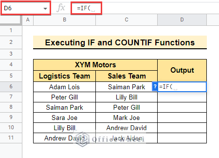
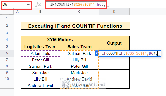
- At first, select cell D6 to enter the functions.

- Now, enter the IF Function to get the desired decision.
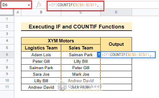
- After that, enter the COUNTIF function to get the output and select the lookup range C6:C11.
- Lock the range to get the exact value from the formula.
- Then, select the lookup value cell B6 and complete the formula.
- Finally, complete the IF function by writing Yes if the value is common in both the team otherwise write Missing and enclose them with double quotes.
=IF(COUNTIF($C$6:$C$11,B6),"Yes","Missing")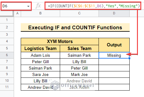
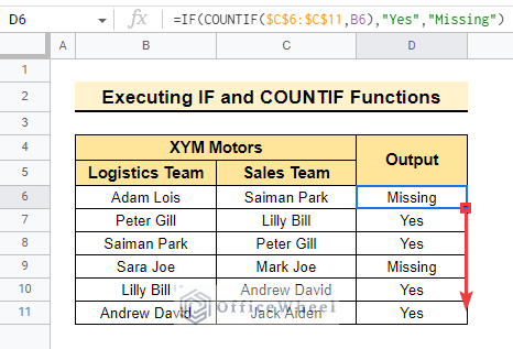
- Now, drag down the fill handle to complete the process.
Read More: How to Use IF Condition Between Two Numbers in Google Sheets
2. Applying ARRAYFORMULA with Multiple Functions
Here, we will apply the ARRAYFORMULA Function along with multiple functions to get if the values are missing or exist in both teams.
📌 Steps:
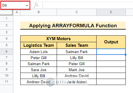
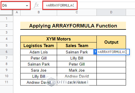
- In the beginning, select cell D6 to enter the formula.
- Then, enter the ARRAYFORMULA Function to combine the values together.
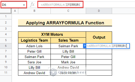
- Therefore, enter the IFERROR function so that the formula returns if there is any error.
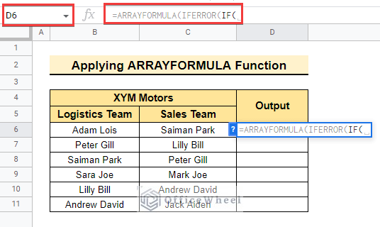
- After that, enter the IF function to get the desired decision in the output.
- Now, enter the MATCH function to match the common value and select range B6:B11 as lookup range and C6:C11 as the result range.
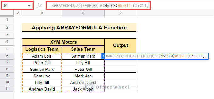
- Finally, complete the MATCH function by writing 0 and complete the IF Function by writing “Yes” manually if the function finds common data otherwise press a blank space.
- In the end, enclose the values with double quotes and the final output is as below.
=ARRAYFORMULA(IFERROR(IF(MATCH(B6:B11,C6:C11,0),"Yes"," ")))
Read More: Generate Random Numbers or Text Between Limits in Google Sheets
Things to Remember
- The Arrayformula function always combines the data if there is more than one column.
- Always use double quotes to enclose the manually written data to execute the function.
Conclusion
In this article, we explained how to find missing values between two columns in google sheets with practical examples. Hopefully, the methods will help you apply these formulas to your dataset. Please let us know in the comment section if you have any further queries or suggestions. You may also visit our OfficeWheel blog to explore more Google Sheets-related articles.
Related Articles
- How to SUMIF Between Two Dates in Google Sheets (3 Ways)
- Find Number of Months Between Two Dates in Google Sheets
- How to Calculate Hours Between Two Times in Google Sheets
- Conditional Formatting Between Two Values in Google Sheets
- How to Insert Lines Between Cells in Google Sheets
- Calculate Percentage Difference Between Two Numbers in Google Sheets
- How to Remove Spaces Between Words in Google Sheets