Sometimes while working on a dataset you need to highlight some specific data so that you get that data quickly. But completing this work manually is nearly impossible or if you manage to do it, it will cost you valuable time. In this case, you can your conditional formatting. Conditional formatting can highlight specific data very quickly. In this article, we will learn how to use conditional formatting between two values in google sheets.
Here is the overview of this article. Hope you will learn more after you go through the whole article below.
A Sample of Practice Spreadsheet
You may copy the spreadsheet below and practice by yourself.
What Is Conditional Formatting in Google Sheets?
While working on Google Sheets, your dataset may contain different types of products. Each category may have unique or duplicate values. The Conditional Formatting feature in Google Sheets allows us to format and highlight datasets properly based on specific rules or criteria. You can apply the Bold, Italic, Underline, and Strikethrough formats, change font colors, and highlight cells based on criteria using this feature.
3 Suitable Ways to Apply Conditional Formatting Between Two Values in Google Sheets
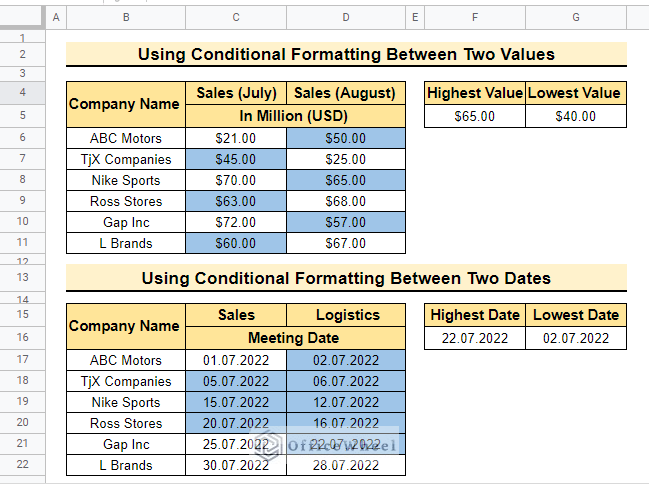
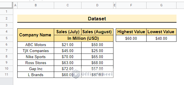
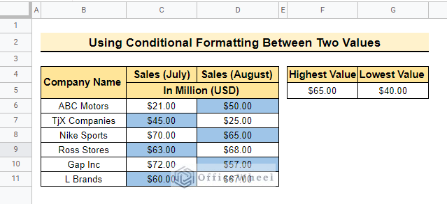
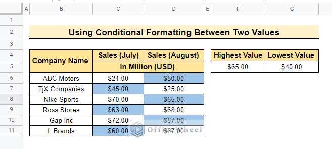
There are 2 types of datasets in this article. The first dataset contains Company Name, Sales for July and August, Highest Value, and Lowest Value. The highest value represents the maximum range of conditional formatting and the lowest value represents the lowest value of conditional formatting. We will conduct the method between these two values. Here we will use conditional formatting between 2 numbers using the following dataset.
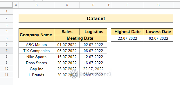
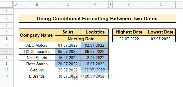
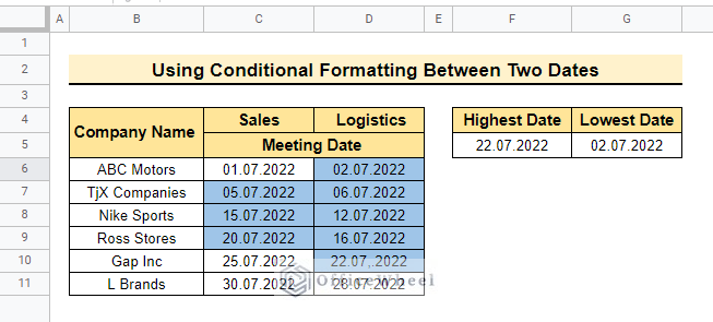
Now, the second dataset contains Company Name, Meeting date of July and August, Highest Value, and Lowest Value. The highest value represents the most previous date and the lowest value represents the most recent date to conduct conditional formatting. We will complete conditional formatting between these two dates. we will use conditional formatting between 2 dates using the following dataset.
1. Applying Is Between Criteria
We will use conditional formatting between two values in google sheets by applying the default Is Between criteria from conditional formatting.
1.1. Between Numbers
Here, we will execute the formula between two numbers.
📌 Steps:
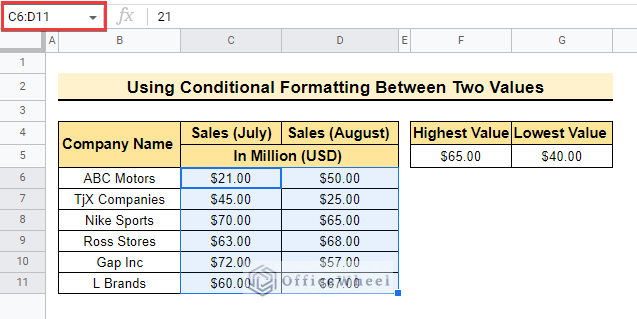
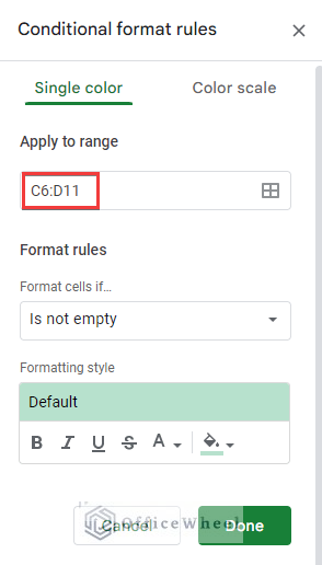
- First, select the range C6:D11 to apply the conditional formatting.
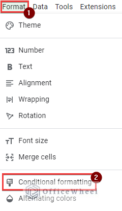
- Then, go to Format >> Conditional formatting from the menu bar.
- After that, Conditional format rules window will pop up with the selected range in Apply to range box.
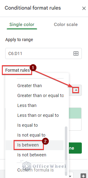
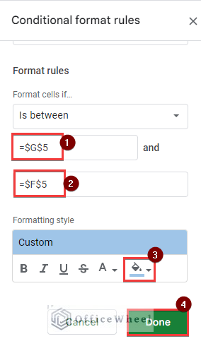
- Now, select Is between from Format rules box as below.
- This option will show two boxes to enter the formula.
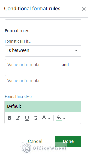
- Here, enter the following formula in the first Value or formula box.
=$G$5- Subsequently, insert the formula below in the last Value or formula box.
=$F$5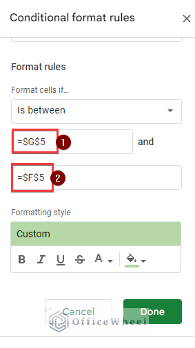
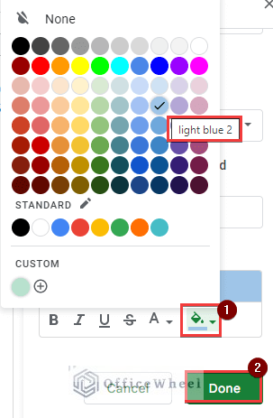
- Now, change the default color from the Formatting style box and click on Done.
- Now, the output will be as below.
Read More: How to Use IF Condition Between Two Numbers in Google Sheets
1.2. Between Dates
We will apply this formula to another dataset that represents the date.
📌 Steps:
- Similarly, complete the first 4 steps already shown in the previous part.
- Now, enter the formula in the first Value or formula box of Conditional rules format window.
=$G$5- Subsequently, insert the formula below in the last Value or formula box and change the color from the Formatting style.
=$F$5- Then click on Done to execute this formula.
- Here, is the output of using the same formula with the same process.

Read More: How to Calculate Time Between Dates in Google Sheets (6 Ways)
Similar Readings
- Difference Between COUNT and COUNTA in Google Sheets
- How to Link Cells Between Tabs in Google Sheets (2 Examples)
- Calculate Number of Years Between Two Dates in Google Sheets
- How to Move Between Tabs in Google Sheets (3 Easy Ways)
- Google Sheets Count Cells Between Two Numbers with COUNTIF Function
2. Using ISBETWEEN Function
Now, we will use conditional formatting between two values using ISBETWEEN Function in the conditional formatting.
2.1. Within Numbers
Moreover, we will use the dataset of numbers to execute this formula.
📌 Steps:
- In the beginning, select the range and select conditional formatting from menu bar as before.
- Therefore, the Conditional format rules box will pop up with the selected range.
- Now, select Custom formula is from Format rules box.
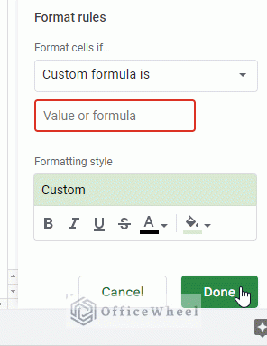
- Now enter the formula in the formula box and change the default color from the Formatting style option.
- After that, select Done to execute the formula.
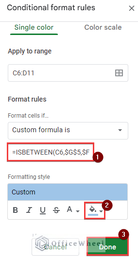
=ISBETWEEN(C6,$G$5,$F$5)
- In the end, the output is below.

Read More: Generate Random Numbers or Text Between Limits in Google Sheets
2.2. Within Dates
Here, we will execute this formula using another dataset that represents date.
📌 Steps:
- In the beginning, complete the initial 4 steps as these steps are similar in this case also.
- Correspondingly, once the Conditional format rules window appears, enter the formula in Values or formula box and change the default color from Formatting style.
=ISBETWEEN(C6,$G$5,$F$5)- Finally, click on Done and complete the process similarly.
- In the end, the final output is below.
Read More: How to SUMIF Between Two Dates in Google Sheets (3 Ways)
Similar Readings
- How to Remove Spaces Between Words in Google Sheets
- Use REGEXEXTRACT Function Between Two Characters in Google Sheets
- How to Find Correlation Between Two Columns in Google Sheets
- Insert Rows Between Other Rows in Google Sheets (4 Easy Ways)
- Find Difference Between Two Columns in Calculated Field of Google Sheets Pivot Table
3. Executing AND Function
Moreover, we will execute the AND Function using both the dataset that represents number and date.
3.1. Between Numbers
we will use conditional formatting between two values applying AND function similarly we applied different procedures before.
📌 Steps:
- First of all, complete all the processes before entering the formula into Value or formula box of Conditional format rules As the process is already shown before.
- Now, enter the AND Function with the following formula and change the default color from Formatting style.
=AND(C6>=$G$5, C6<=$F$5)- Finally, click Done to execute the formula.
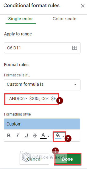
- In the end, the final output will be as follows.
Read More: Calculate Percentage Difference Between Two Numbers in Google Sheets
3.2. Between Dates
Now, we will apply the same formula using another dataset that contains a value representing the date.
📌 Steps:
- As the first 4 steps are the same in every process, complete all the similar steps which are shown before.
- After that, enter the formula below in Value or formula box, once the Conditional formatting rules window appears.
- Subsequently, change the default color from Formatting style option, so that the formatting is more visible.
=AND(C6>=$G$5, C6<=$F$5)- Then, click on Done to execute this formula.

- Finally, the output is as follows.
Read More: How to Filter Between Two Dates in Google Sheets
Things to Remember
- Always remember to enter the correct formula otherwise it will highlight wrong values.
- Formate cells if represents condition so you can use any condition to execute conditional formatting.
Conclusion
In this article, we explained how to use conditional formatting between two values in google sheets with practical examples. Hopefully, the methods will help you to apply these formulas to your own dataset. Please let us know in the comment section if you have any further queries or suggestions. You may also visit our OfficeWheel blog to explore more Google Sheets-related articles.